시작점에서 출발

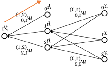
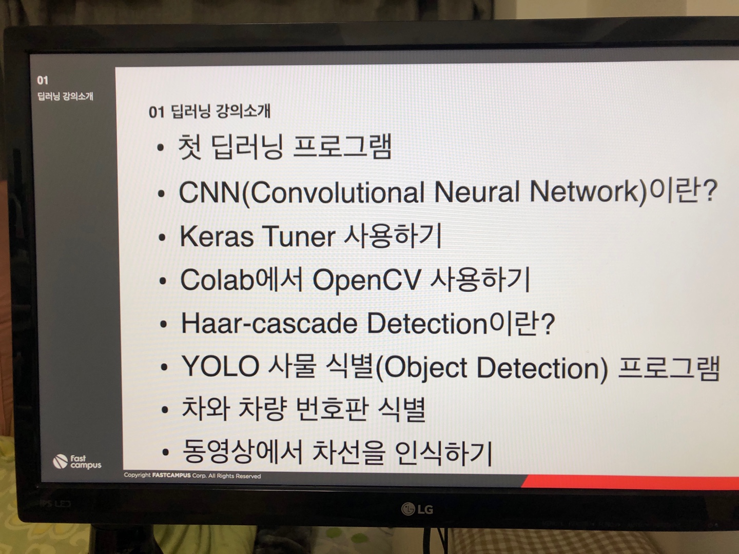
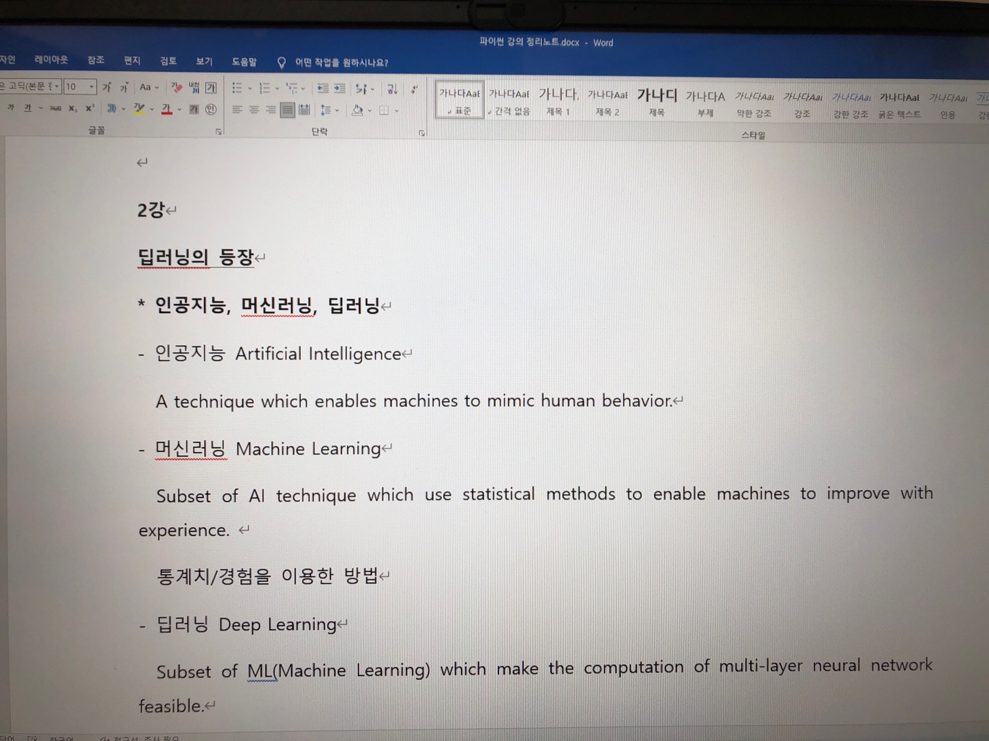
파이썬 기초부터 시작하는 딥러닝 영상 인식 바이블 Online강의를 50일간 수강했다. 

파이썬 기초 강의 14강
데이터 분석 강의 32강
머신러닝 강의 25강
딥러닝 영상처리 강의 39강
자율주행 영상인식 강의 29강

총 139강으로 이루어져 있고, 한 강의에 최대 40분을 넘기지 않아 총 57시간 25분이 소요되는 구성이다.

이렇게 정리해보니 사실 그렇게 긴 강의도 아닌데 아직 완강을 하지 못했다.

직장 다니면서 강의 듣는게 뭐 그리 어렵겠냐고 쉽게 생각했는데, 막상 내가 강의를 들을 일이 생기고 여건이 따라주지 않으니 이런 결과가 생긴 것 같다.

50일간 하루도 빠지지 않고 한시간 정도씩 들었으면 아마 완강이 가능하지 않았을까 하고 생각한다.

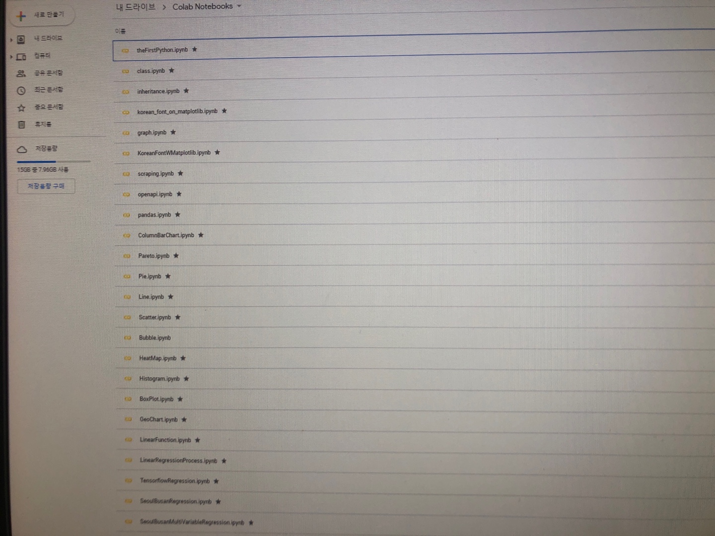
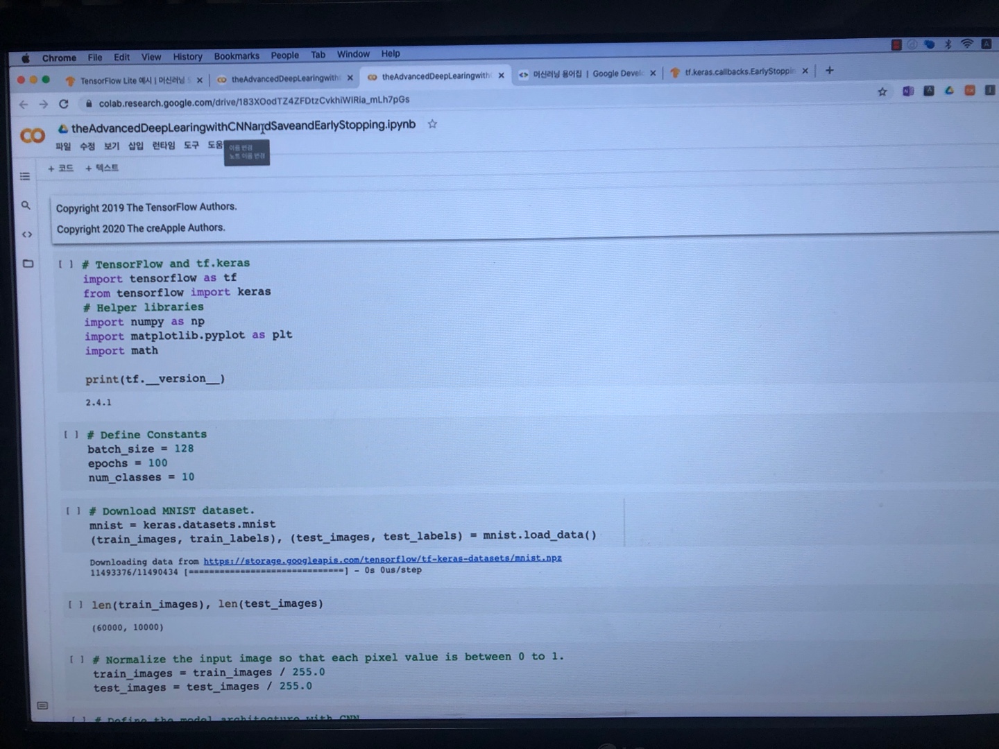
그동안 강의를 들으면서 생성한 Colab 파일이 이만큼 쌓였다. 

쌓여있는 기록을 보면 그래도 내가 그동안 놀지는 않았구나 하는 생각은 든다.

비록 투자한 시간이 아주 길지는 않지만 내 하루의 단 몇 분이라도 강의를 듣는데 썼음에 의의를 두고싶다.

파이썬 기초강의

파이썬 기초강의 부분은 가장 따라가기 쉬웠던 부분이다. 

이 부분을 하루에 여러 강 학습하였으면 더 좋았을 거라고 생각한다.

이전에도 파이썬을 공부한 적은 있지만, 따로 강의를 듣거나 교재가 있었던 것이 아니라 인터넷에서 이부분 저부분을 따라하는 수준이었고 그나마도 안 쓰는 동안 많이 잊어버렸었다.

그래서 기본 문법을 다시 정리하기 좋았다.

다만, 가끔 강사님 코드대로 따라 적어도 에러가 발생하는 경우가 있어서 그 때에는 알아서 구글링을 통해 에러를 수정해야했다. 

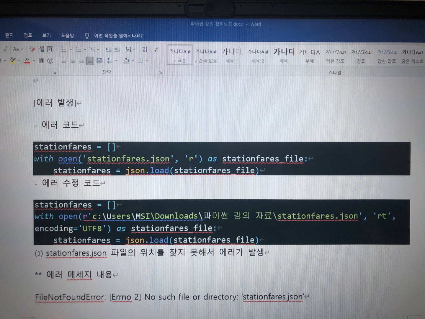
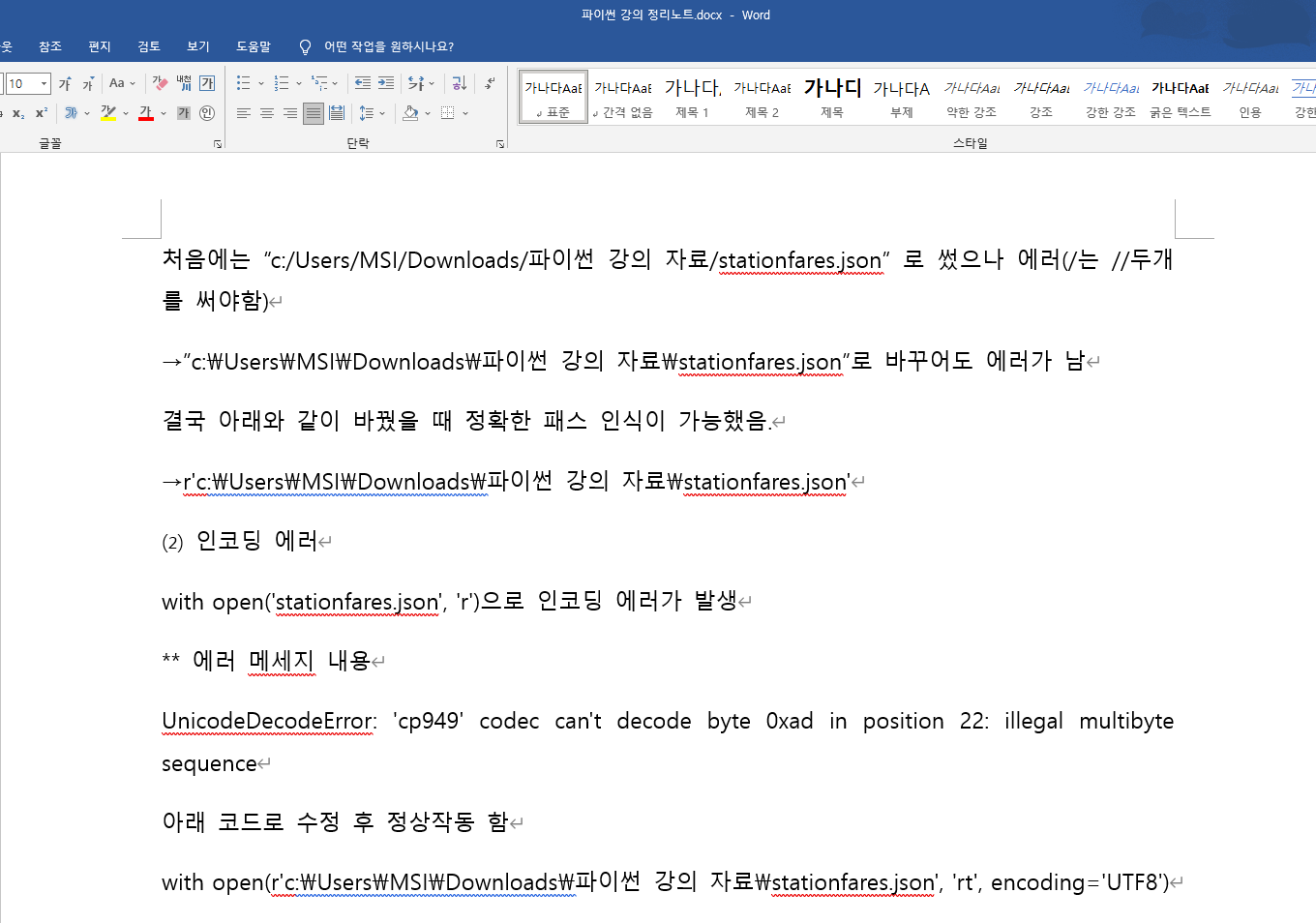
⑴ stationfares.json 파일의 위치를 찾지 못해서 에러가 발생
** 에러 메세지 내용
FileNotFoundError: [Errno 2] No such file or directory: 'stationfares.json'
처음에는 “c:/Users/MSI/Downloads/파이썬 강의 자료/stationfares.json” 로 썼으나 에러(/는 //두개를 써야함)
→”c:\Users\MSI\Downloads\파이썬 강의 자료\stationfares.json”로 바꾸어도 에러가 남
결국 아래와 같이 바꿨을 때 정확한 패스 인식이 가능했음.
→r'c:\Users\MSI\Downloads\파이썬 강의 자료\stationfares.json'

⑵ 인코딩 에러
with open('stationfares.json', 'r')으로 인코딩 에러가 발생
** 에러 메세지 내용
UnicodeDecodeError: 'cp949' codec can't decode byte 0xad in position 22: illegal multibyte sequence
아래 코드로 수정 후 정상작동 함
with open(r'c:\Users\MSI\Downloads\파이썬 강의 자료\stationfares.json', 'rt', encoding='UTF8')

데이터 분석 강의

데이터 분석강의는 Matplotlib라이브러리를 통해 그래프로 데이터를 시각화하는 파트였다.

Colab에서 한글 인코딩이 안되서 강사님이 폰트 설치 방법부터 셋팅하는 방법까지 다 알려주셨는데, 

처음에는 그 순서 그대로 다 따라해도 인코딩 에러가 나서 강의가 끝나고 나서도 계속 구글에서 에러 원인이랑 해결방법을 검색했던 것이 생각난다. 

그리고 그렇게 했는데도 해결이 안되서 다음 날 수강 때 강사님 방법대로 다시 따라했는데 에러가 안 났다.

아마 인덴트 에러였거나 내가 처음에 실행했던 순서가 문제가 있었던게 아닐까 생각한다. 

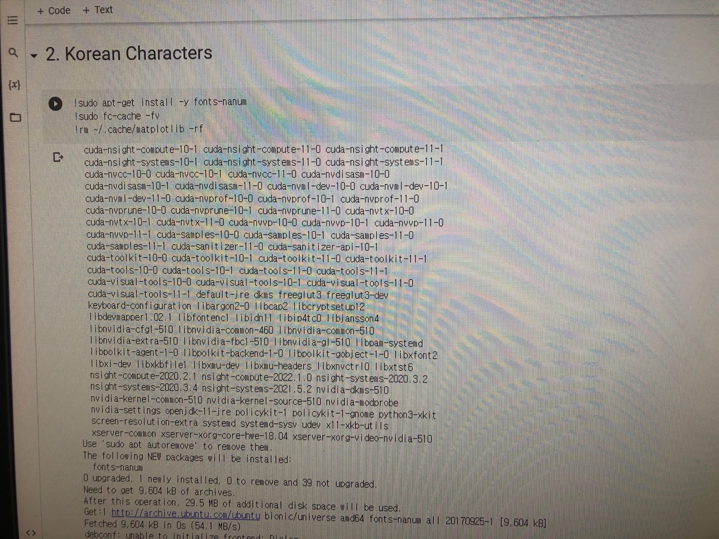
이 파트에서부터 루틴처럼 쓰이는 코드가 있다. 

1. Mount Drive(Google Drive 연결)

from google.colab import drive

drive.mount('/gdrive')

2. Korean Encoding

!sudo apt-get install -y fonts-nanum

!sudo fc-cache -fv

!rm ~/.cache/matplotlib -rf

** Runtime Restart → 필요한 코드 재시작

3. Matplotlib

# Import pyplot as a alias 'plt'

import matplotlib.pyplot as plt

# 폰트를 Nanum폰트로 지정

plt.rc('font', family='NanumBarunGothic')

4. Load Data

# Load a file under "data" folder

file = "/gdrive/My Drive/data/data_2021.csv"

import pandas as pd

data = pd.read_csv(file)

이 파트에서 좋았던 점이 좀 많았다.

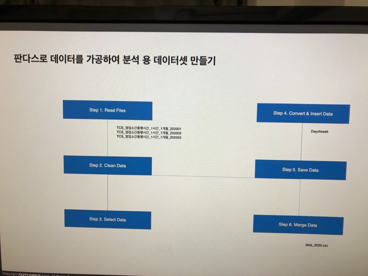
• 데이터 셋 작성 방법
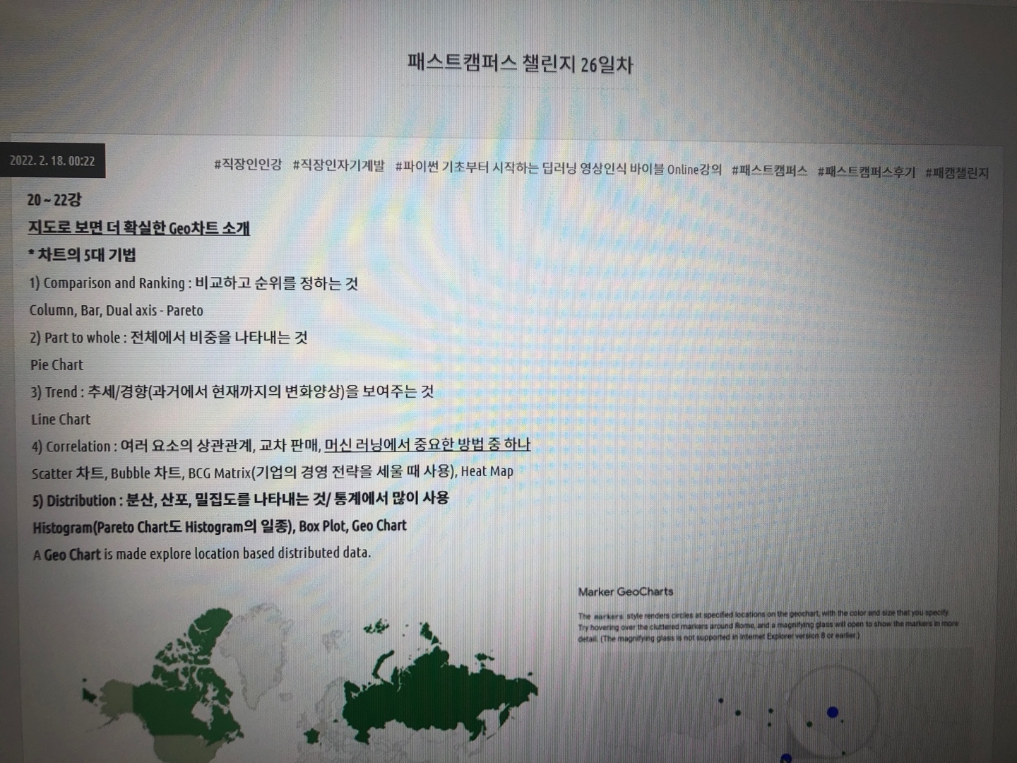
• 차트의 5대 기법
• 데이터 시각화
• API사용 방법

이 파트에서 여러 그래프를 구현해 보는 것은 재미있는 경험이었다. 

다만 강사님이 강의를 녹화한 시점과 실제로 강의를 듣는 시점의 시간차가 있어서 데이터 결과 값이 다르니 내가 강사님을 따라 구현한 것이 정확한지 확인할 수 없다는 부분은 아쉬웠다. 

또한 각 그래프의 특성에 맞는 데이터가 따로 있기 때문에 그 특성을 잘 나타내기 힘든 데이터를 이용하는 것 보다는 각 그래프마다 사용할 특정 데이터를 제공하여 해당 데이터를 데이터셋으로 가공하는 강의가 더 좋지 않을까하고 생각해봤다. 

머신러닝 강의

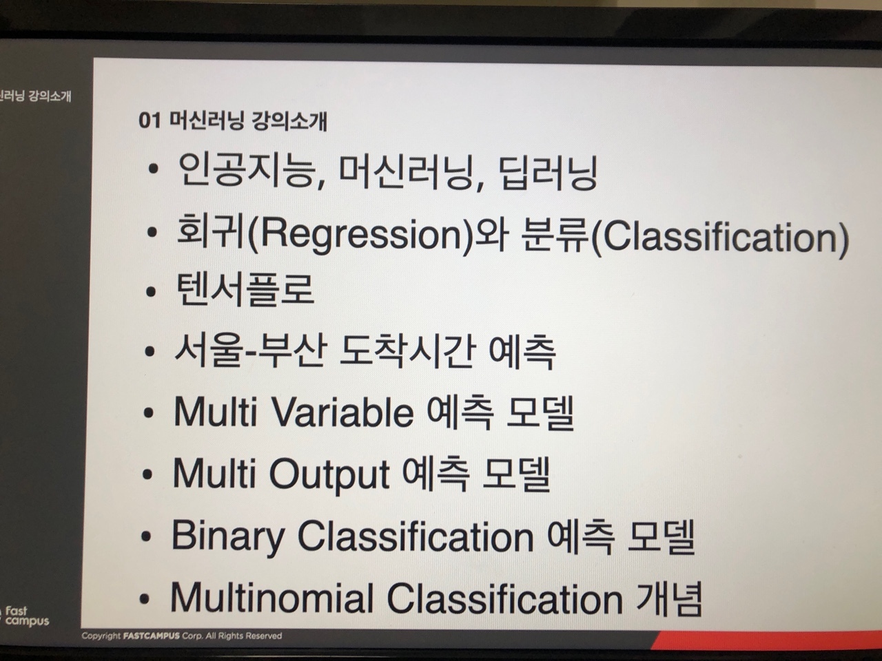
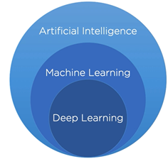
인공지능, 머신러닝, 딥러닝의 개념을 정리하고 머신러닝의 기본을 배울 수 있는 강의이다. 

머신러닝 강의에서부터는 한 강의 시간이 짧아도 그 강의 시간 내에 이해가 다 안 되서 강의를 계속 다시 돌려봤던 것 같다.  강의 내내 토끼와 거북이 이야기를 통해 머신러닝에 대해 알려주시는데 최대한 쉽게 설명하려고 하시는게 느껴졌다.  하지만 한 번만 들어서는 잘 이해가 안 가서 아마 완강 후에도 2, 3번은 더 들어야 할 것 같다.

머신러닝 강의에서부터 Tensorflow를 사용하기 시작한다.

기본적으로 아래 코드의 틀에서 크게 벗어나지 않는 선에서 조금씩 필요한 부분을 변경해서 강의를 하신다.

모델링 할 때 사용하는 최적화 방법과 Squared Error방식에 대해서 여러 번 설명해주시는데 내 강의 이해력의 문제로 아직 정확하게 이해하지 못한 것 같다. 

딥러닝 영상처리 강의

딥러닝 영상처리 강의의 첫 부분은 MNIST의 데이터를 이용하여 이미지 속의 숫자를 인식하는 걸로 시작한다.

그리고 Keras, ReLu를 좀 더 자세하게 다룬다.

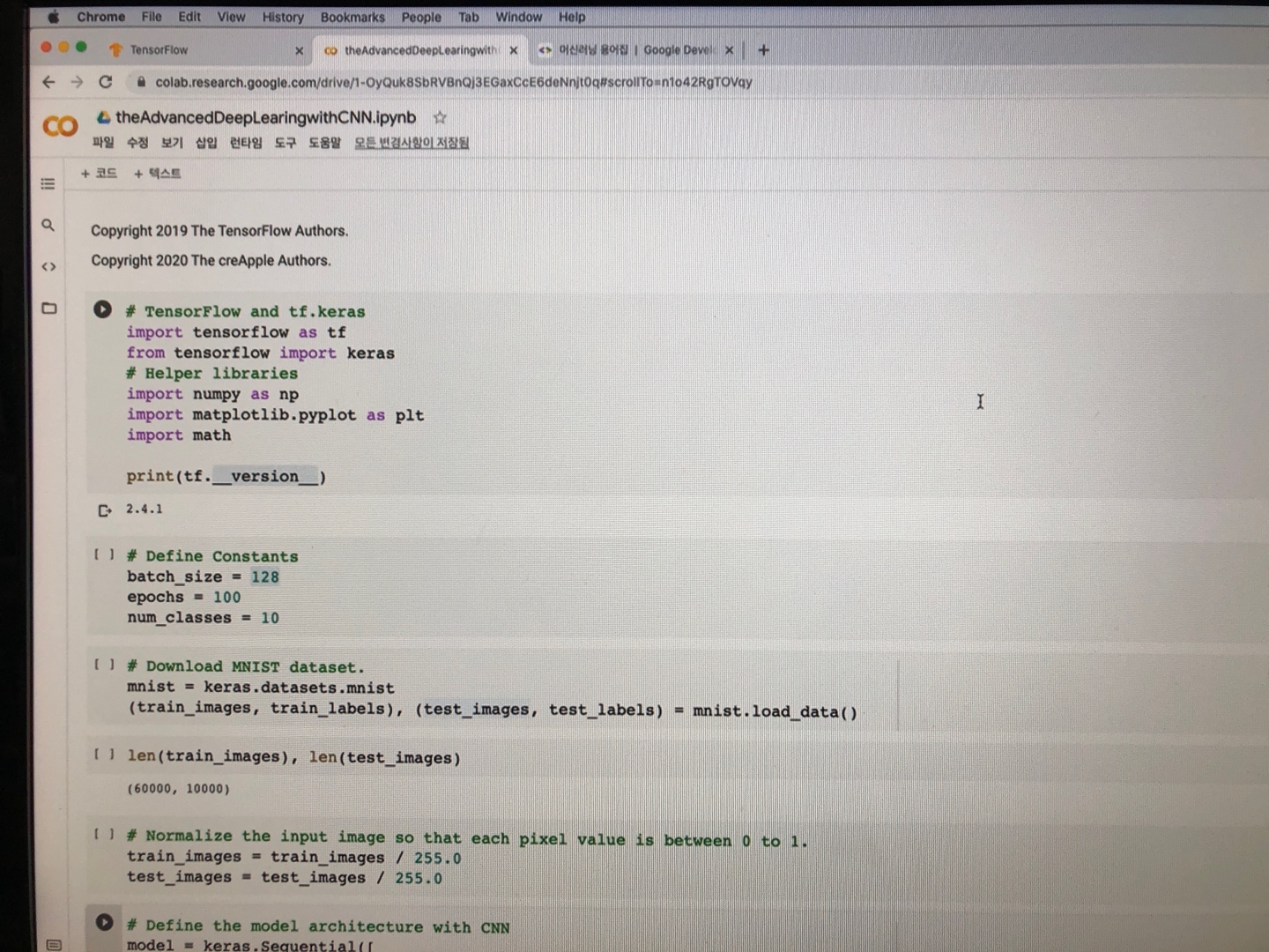
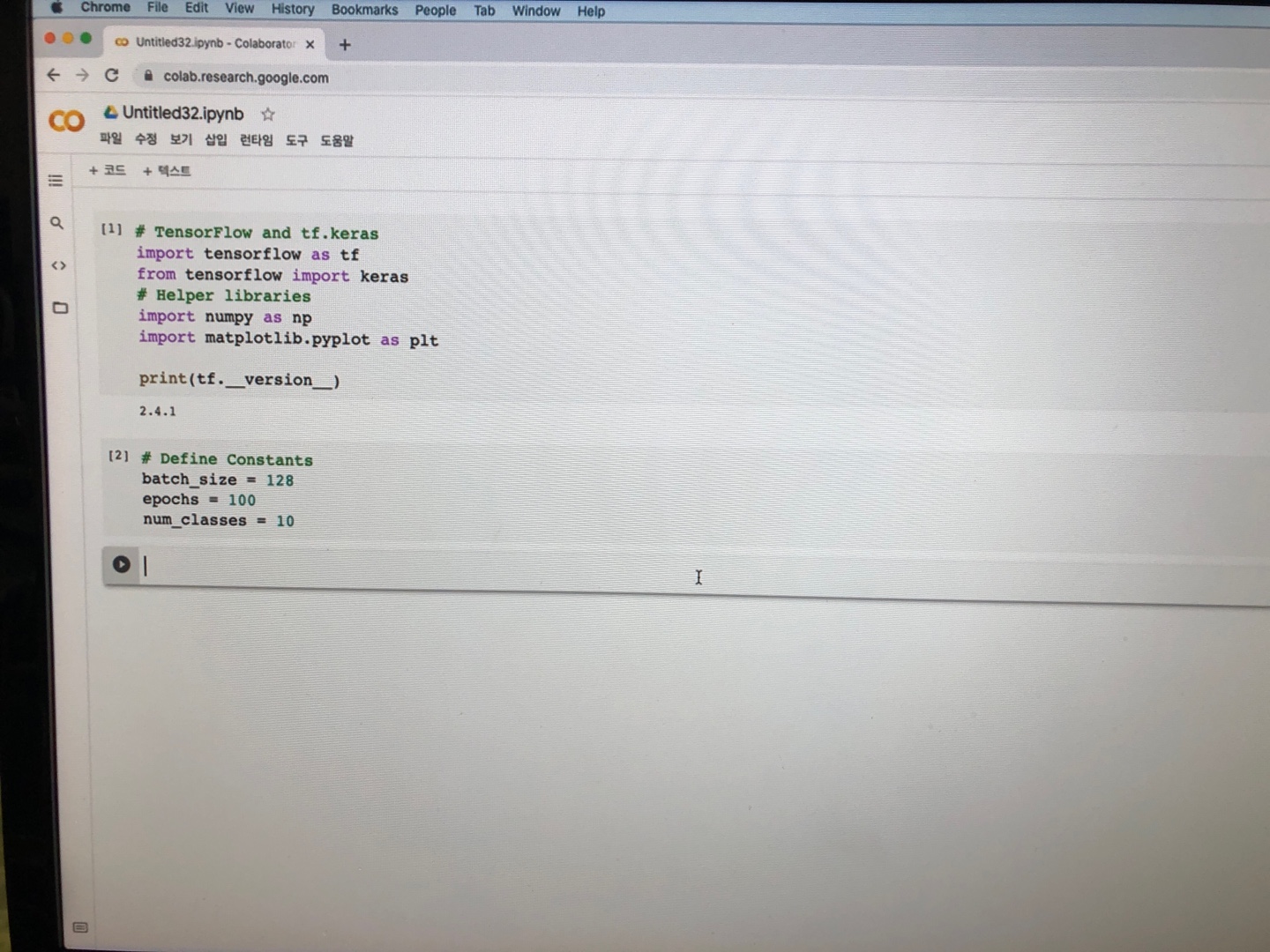
필요한 라이브러리 인포트

# TensorFlow and tf.keras

import tensorflow as tf

from tensorflow import keras

# Helper libraries

import numpy as np

import matplotlib.pyplot as plt

import math

상수 선언

# Define Constants

batch_size = 128

epochs = 10000

num_classes = 10

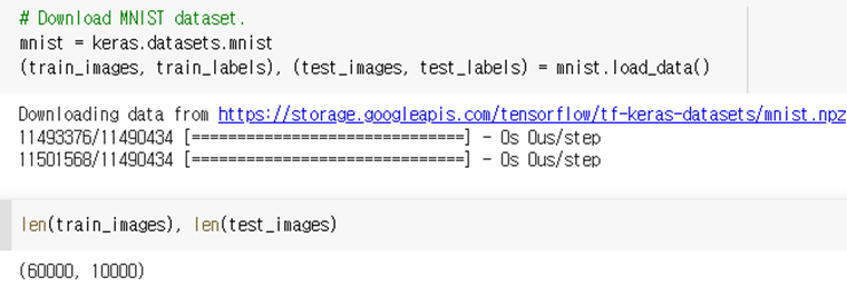
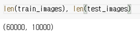
MNIST에서 학습용(6만개), 테스트용(1만개) 이미지 셋(이미지, 결과 값 페어) 다운로드

# Download MNIST dataset.

mnist = keras.datasets.mnist

(train_images, train_labels), (test_images, test_labels) = mnist.load_data()

Tensorflow에서 계산하기 쉽도록 값을 0에서 1사이의 값으로 변환 계산한다.

** 각 이미지에는 0~ 255까지의 채도 값이 들어있다.

# Normalize the input image so that each pixel value is between 0 to 1.

train_images = train_images / 255.0

test_images = test_images / 255.0

모델 생성

** 모델을 견고하게 변경, 은닉층을 보강, Convolutional Neural Network를 이용해서 강화

# Define the model architecture with CNN

model = keras.Sequential([

                         keras.layers.Flatten(input_shape=(28,28)),

                         # Hidden Layers

                         # keras.layers.Dense(128, activation=tf.nn.relu),

                         keras.layers.Reshape(target_shape=(28, 28, 1)),

                         keras.layers.Conv2D(filters=32, kernel_size=(3, 3), activation=tf.nn.relu),

                         keras.layers.Conv2D(filters=64, kernel_size=(3, 3), activation=tf.nn.relu),

                         keras.layers.MaxPooling2D(pool_size=(2, 2)),

                         keras.layers.Dropout(0.25),

                         keras.layers.Flatten(input_shape=(28, 28)),

                         keras.layers.Dense(128, activation=tf.nn.relu),

                         keras.layers.Dropout(0.5),

                         keras.layers.Dense(num_classes, activation='softmax')

])

model.compile(optimizer='adam',

              loss=tf.keras.losses.SparseCategoricalCrossentropy(from_logits=True),

              metrics=['accuracy'])

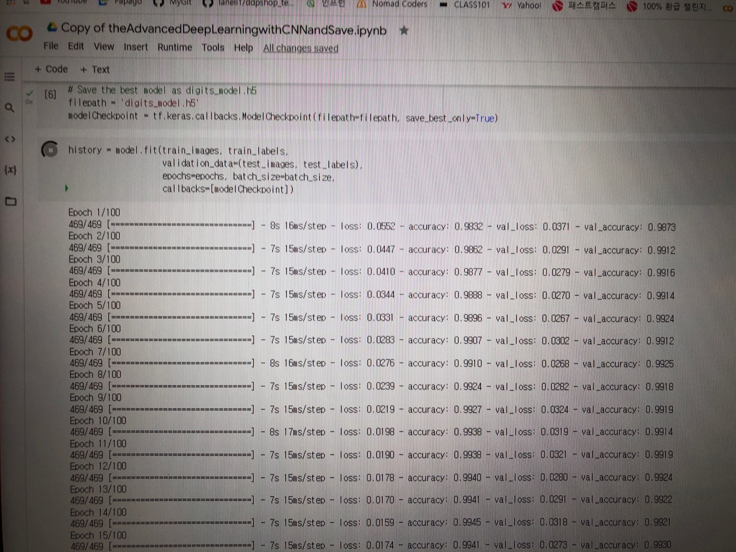
모델 체크포인트 객체 생성

# Save the best model as digits_model.h5

filepath = 'digits_model.h5'

modelCheckpoint = tf.keras.callbacks.ModelCheckpoint(filepath=filepath, save_best_only=True)

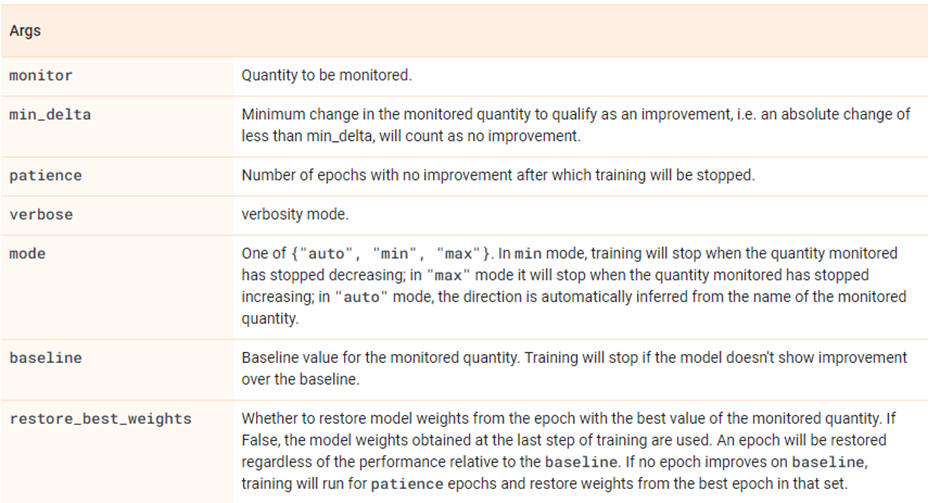
Early Stopping 작성 : 모니터링 대상은 validation loss값이다.

# Define a callback to monitor val_loss

monitorEarlyStop = tf.keras.callbacks.EarlyStopping(monitor='val_loss', patience=5)

[참고]

https://www.tensorflow.org/api_docs/python/tf/keras/callbacks/EarlyStopping

** monitor : 모니터 대상

** patience : local minimum이 있을 수 있기 때문에, 정해 놓은 횟수 만큼은 기다리는 것이다.

학습 : callback 설정

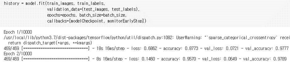
history = model.fit(train_images, train_labels,

                    validation_data=(test_images, test_labels),

                    epochs=epochs, batch_size=batch_size,

                    callbacks=[modelCheckpoint, monitorEarlyStop])

자율주행 영상 강의

아직 딥러닝 영상처리 강의 부분을 수강하는 중이라 자율주행 영상강의에 대한 정보가 없다. 

아마 완강을 하게되면 이 후기 부분을 수정하는 형식이 되지 않을까한다.

모든 수강생의 수준이 같지 않기때문에 100프로 만족하는 강의를 찾는 것은 어려울 것이라고 생각한다. 

하지만 이번 파이썬 기초부터 시작하는 딥러닝 영상 인식 바이블 Online강의는 100프로는 아니라도 80%는 만족하는 강의였다. 필요한 부분을 두번, 세번 반복해서 들으면 더 좋은 강의인 것 같다. 

그리고 한 강의에 할당해야하는 시간이 길어도 30분을 넘기지 않아서 부담스럽지 않다. 

이후 되도록 빨리 남은 강의를 완강하는게 목표이다. 

완강 후에는 자율주행 영상 처리에 대해 얕게나마 지식이 쌓여있기를 바란다.

기재: 본 포스팅은 패스트캠퍼스 환급 챌린지 참여를 위해 작성되었습니다.

https://bit.ly/37BpXiC

9강

모델 Early Stopping

모델이 훈련 세트에서 적절한 패턴을 학습하여 모델 성능이 최고점에 도달한 경우 자동으로 학습을 종료해주는 것. Early Stopping을 사용하면 정해놓은 epochs의 횟수만큼 다 학습을 하는 것이 아니라 학습 도중 모니터 하고 있는 값이 모니터 하는 도중 개선효과가 없어지기 시작하면 학습을 중단한다.

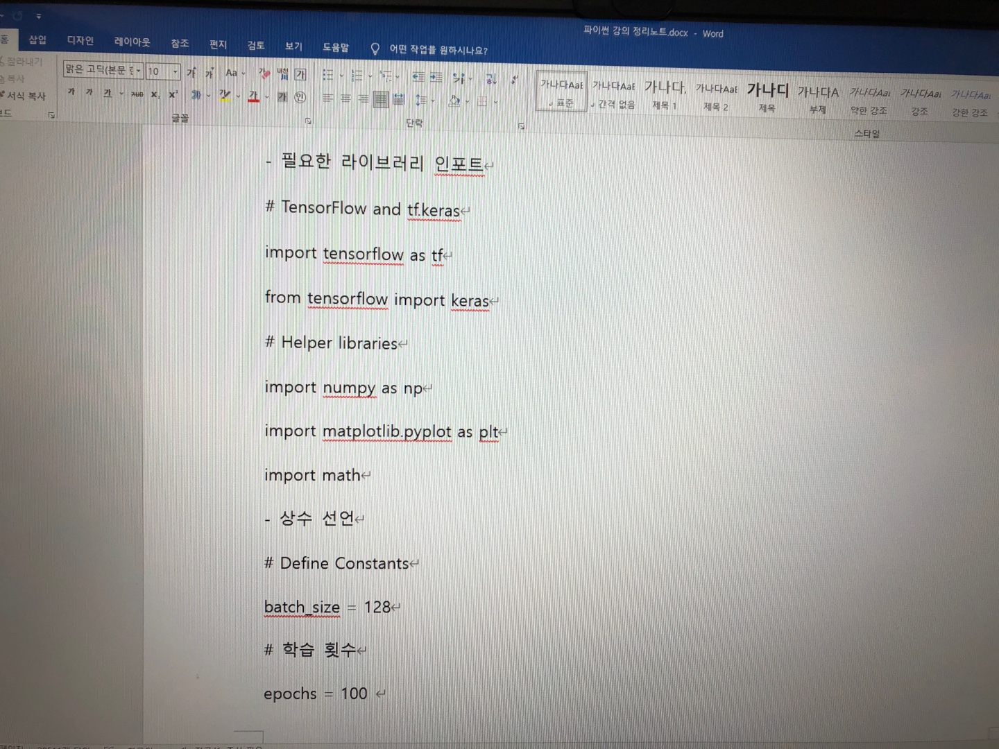
- 필요한 라이브러리 인포트

# TensorFlow and tf.keras

import tensorflow as tf

from tensorflow import keras

# Helper libraries

import numpy as np

import matplotlib.pyplot as plt

import math

- 상수 선언

# Define Constants

batch_size = 128

epochs = 10000

num_classes = 10

- MNIST에서 학습용(6만개), 테스트용(1만개) 이미지 셋(이미지, 결과 값 페어) 다운로드

# Download MNIST dataset.

mnist = keras.datasets.mnist

(train_images, train_labels), (test_images, test_labels) = mnist.load_data()

- Tensorflow에서 계산하기 쉽도록 값을 0에서 1사이의 값으로 변환 계산한다.

 : 실수로 계산하는 것이 더 좋다.

** 각 이미지에는 0~ 255까지의 채도 값이 들어있다.

# Normalize the input image so that each pixel value is between 0 to 1.

train_images = train_images / 255.0

test_images = test_images / 255.0

- 모델 생성

** 모델을 견고하게 변경, 은닉층을 보강, Convolutional Neural Network를 이용해서 강화

# Define the model architecture with CNN

model = keras.Sequential([

                         keras.layers.Flatten(input_shape=(28,28)),

                         # Hidden Layers

                         # keras.layers.Dense(128, activation=tf.nn.relu),

                         keras.layers.Reshape(target_shape=(28, 28, 1)),

                         keras.layers.Conv2D(filters=32, kernel_size=(3, 3), activation=tf.nn.relu),

                         keras.layers.Conv2D(filters=64, kernel_size=(3, 3), activation=tf.nn.relu),

                         keras.layers.MaxPooling2D(pool_size=(2, 2)),

                         keras.layers.Dropout(0.25),

                         keras.layers.Flatten(input_shape=(28, 28)),

                         keras.layers.Dense(128, activation=tf.nn.relu),

                         keras.layers.Dropout(0.5),

                         keras.layers.Dense(num_classes, activation='softmax')

])

model.compile(optimizer='adam',

              loss=tf.keras.losses.SparseCategoricalCrossentropy(from_logits=True),

              metrics=['accuracy'])

- 모델 체크포인트 객체 생성

# Save the best model as digits_model.h5

filepath = 'digits_model.h5'

modelCheckpoint = tf.keras.callbacks.ModelCheckpoint(filepath=filepath, save_best_only=True)

- Early Stopping 작성 : 모니터링 대상은 validation loss값이다.

# Define a callback to monitor val_loss

monitorEarlyStop = tf.keras.callbacks.EarlyStopping(monitor='val_loss', patience=5)

[참고]

https://www.tensorflow.org/api_docs/python/tf/keras/callbacks/EarlyStopping

** monitor : 모니터 대상

** patience : local minimum이 있을 수 있기 때문에, 정해 놓은 횟수 만큼은 기다리는 것이다.

- 학습 : callback 설정

history = model.fit(train_images, train_labels,

                    validation_data=(test_images, test_labels),

                    epochs=epochs, batch_size=batch_size,

                    callbacks=[modelCheckpoint, monitorEarlyStop])

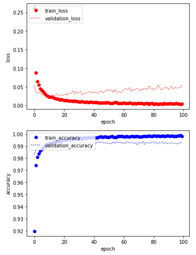
** val_loss의 값이 낮아지는 동안에는 멈추지 않는다.

** 총 16회 학습했다.

- 그림 표시용 함수 선언

# Helper function to display digit images

# 샘플을 보여주는 함수

def show_sample(images, labels, sample_count=25):

  # Create a square with can fit {sample_count} images

  grid_count = math.ceil(math.ceil(math.sqrt(sample_count)))

  grid_count = min(grid_count, len(images), len(labels))

  plt.figure(figsize=(2*grid_count, 2*grid_count))

  for i in range(sample_count):

    plt.subplot(grid_count, grid_count, i+1)

    plt.xticks([])

    plt.yticks([])

    plt.grid(False)

    plt.imshow(images[i], cmap=plt.cm.gray)

    plt.xlabel(labels[i])

  plt.show()

# Helper function to display specific digit images

# 샘플의 특정 숫자를 보여주는 함수

def show_sample_digit(images, labels, digit, sample_count=25):

  # Create a square with can fit {sample_count} images

  grid_count = math.ceil(math.ceil(math.sqrt(sample_count)))

  grid_count = min(grid_count, len(images), len(labels))

  plt.figure(figsize=(2*grid_count, 2*grid_count))

  i = 0

  digit_count = 0

  while digit_count < sample_count:

    i += 1

    if (digit == labels[i]):

      plt.subplot(grid_count, grid_count, digit_count+1)

      plt.xticks([])

      plt.yticks([])

      plt.grid(False)

      plt.imshow(images[i], cmap=plt.cm.gray)

      plt.xlabel(labels[i])

      digit_count += 1

  plt.show()

# Helper function to display specific digit images

# 특정 숫자를 좀 더 크게 보여주는 함수

def show_digit_image(image):

  # Draw digit image

  fig = plt.figure()

  ax = fig.add_subplot(1, 1, 1)

  # Major ticks every 20, minor ticks every 5

  major_ticks = np.arange(0, 29, 5)

  minor_ticks = np.arange(0, 29, 1)

  ax.set_xticks(major_ticks)

  ax.set_xticks(minor_ticks, minor=True)

  ax.set_yticks(major_ticks)

  ax.set_yticks(minor_ticks, minor=True)

  # And a corresponding grid

  ax.grid(which='both')

  # Or if you want different settings for the grids:

  ax.grid(which='minor', alpha=0.2)

  ax.grid(which='major', alpha=0.5)

  ax.imshow(image, cmap=plt.cm.binary)

plt.show()

# 다운로드 하는 함수

# Download the digit classification model if you're using Colab,

# or print the model's local path if you're not using Colab.

def download(path):

    try:

        from google.colab import files

        files.download(path)

    except ImportError:

        import os

        print('Error dowbload:', os.path.join(os,getcwd(), path))

- 모델 다운로드

# Download the digit classification model if you're using Colab

download(filepath)

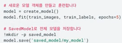
- 전체 모델 저장

# Save Model

savefile = 'saved_digits.h5'

model.save(savefile)

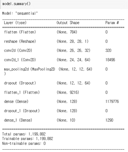
- 모델 구조 확인

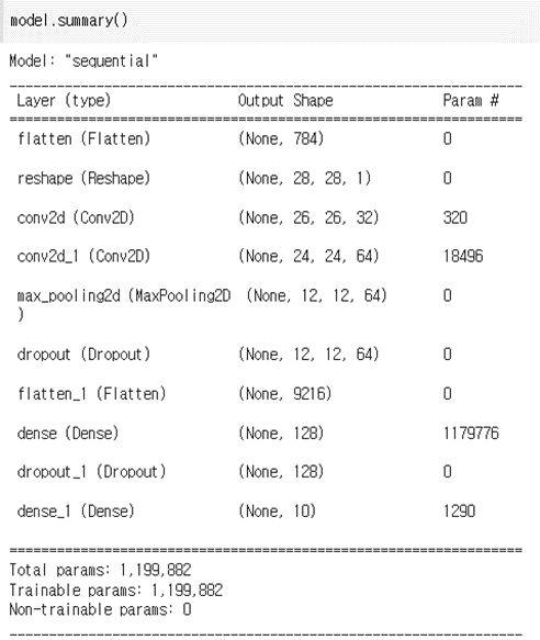
model.summary()

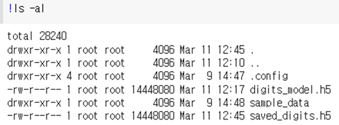
- 저장된 내용 확인(리눅스 명령어)

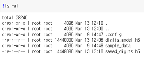
!ls -al

- 모델 불러오기

# Load Model

load_model = tf.keras.models.load_model(savefile)

- 불러온 모델 구조 확인

load_model.summary()

- 모델 정확도 평가

# Evaluate the model using test dataset.

test_loss, test_acc = model.evaluate(test_images, test_labels)

print('Test Accuracy: ', test_acc)

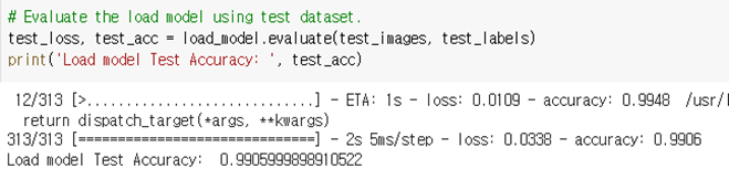
# Evaluate the load model using test dataset.

test_loss, test_acc = load_model.evaluate(test_images, test_labels)

print('Load model Test Accuracy: ', test_acc)

- 그래프 생성

# Evaluate the model using test dataset. - Show performance

fig, loss_ax = plt.subplots()

fig, acc_ax = plt.subplots()

loss_ax.plot(history.history['loss'], 'ro', label='train_loss')

loss_ax.plot(history.history['val_loss'], 'r:', label='validation_loss')

loss_ax.set_xlabel('epoch')

loss_ax.set_ylabel('loss')

loss_ax.legend(loc='upper left')

acc_ax.plot(history.history['accuracy'], 'bo', label='train_accuracy')

acc_ax.plot(history.history['val_accuracy'], 'b:', label='validation_accuracy')

acc_ax.set_xlabel('epoch')

acc_ax.set_ylabel('accuracy')

acc_ax.legend(loc='upper left')

plt.show()

기재: 본 포스팅은 패스트캠퍼스 환급 챌린지 참여를 위해 작성되었습니다.

https://bit.ly/37BpXiC

8강

모델 저장 및 로드

[참조]

https://www.tensorflow.org/tutorials/keras/save_and_load

훈련하는 도중이나 훈련이 끝난 후에 모델을 저장할 수 있습니다. 모델을 중지된 지점부터 다시 훈련할 수 있어 한 번에 오랫동안 훈련하지 않아도 됩니다. 또 모델을 저장하면 다른 사람에게 공유할 수 있고 작업을 재현할 수 있습니다.

저장한 모델로 웹서비스를 제공할 수 있다.

- 필요한 라이브러리 인포트

# TensorFlow and tf.keras

import tensorflow as tf

from tensorflow import keras

# Helper libraries

import numpy as np

import matplotlib.pyplot as plt

import math

- 상수 선언

# Define Constants

batch_size = 128

epochs = 100

num_classes = 10

- MNIST에서 학습용(6만개), 테스트용(1만개) 이미지 셋(이미지, 결과 값 페어) 다운로드

# Download MNIST dataset.

mnist = keras.datasets.mnist

(train_images, train_labels), (test_images, test_labels) = mnist.load_data()

- Tensorflow에서 계산하기 쉽도록 값을 0에서 1사이의 값으로 변환 계산한다.

 : 실수로 계산하는 것이 더 좋다.

** 각 이미지에는 0~ 255까지의 채도 값이 들어있다.

# Normalize the input image so that each pixel value is between 0 to 1.

train_images = train_images / 255.0

test_images = test_images / 255.0

- 모델 생성

** 모델을 견고하게 변경, 은닉층을 보강, Convolutional Neural Network를 이용해서 강화

# Define the model architecture with CNN

model = keras.Sequential([

                         # Input Layer

                         keras.layers.Flatten(input_shape=(28,28)),

# Hidden Layers

                         keras.layers.Reshape(target_shape=(28, 28, 1)),

                         keras.layers.Conv2D(filters=32, kernel_size=(3, 3), activation=tf.nn.relu),

                         keras.layers.Conv2D(filters=64, kernel_size=(3, 3), activation=tf.nn.relu),

                         keras.layers.MaxPooling2D(pool_size=(2, 2)),

                         keras.layers.Dropout(0.25),

                         keras.layers.Flatten(input_shape=(28, 28)),

                         keras.layers.Dense(128, activation=tf.nn.relu),

                         keras.layers.Dropout(0.5),

                         # Output Layer

                         keras.layers.Dense(num_classes, activation='softmax')

])

model.compile(optimizer='adam',

              loss=tf.keras.losses.SparseCategoricalCrossentropy(from_logits=True),

              metrics=['accuracy'])

** 체크포인트 콜백 매개변수 callbacks

이 콜백 함수는 몇 가지 매개변수를 제공합니다. 체크포인트 이름을 고유하게 만들거나 체크포인트 주기를 조정할 수 있습니다.

<새로운 모델을 훈련하고 에포크마다 고유한 이름으로 체크포인트를 저장하는 예제>

- 모델 체크포인트 객체 생성

# Save the best model as digits_model.h5

filepath = 'digits_model.h5'

modelCheckpoint = tf.keras.callbacks.ModelCheckpoint(filepath=filepath, save_best_only=True)

- 학습 : callback 설정

history = model.fit(train_images, train_labels,

                    validation_data=(test_images, test_labels),

                    epochs=epochs, batch_size=batch_size,

                    callbacks=[modelCheckpoint])

** callbacks=[] : 리스트인 경우 값이 복수 개, 단수 개의 값을 넣을 수도 있다.

- 그림 표시용 함수 선언

# Helper function to display digit images

# 샘플을 보여주는 함수

def show_sample(images, labels, sample_count=25):

  # Create a square with can fit {sample_count} images

  grid_count = math.ceil(math.ceil(math.sqrt(sample_count)))

  grid_count = min(grid_count, len(images), len(labels))

  plt.figure(figsize=(2*grid_count, 2*grid_count))

  for i in range(sample_count):

    plt.subplot(grid_count, grid_count, i+1)

    plt.xticks([])

    plt.yticks([])

    plt.grid(False)

    plt.imshow(images[i], cmap=plt.cm.gray)

    plt.xlabel(labels[i])

  plt.show()

# Helper function to display specific digit images

# 샘플의 특정 숫자를 보여주는 함수

def show_sample_digit(images, labels, digit, sample_count=25):

  # Create a square with can fit {sample_count} images

  grid_count = math.ceil(math.ceil(math.sqrt(sample_count)))

  grid_count = min(grid_count, len(images), len(labels))

  plt.figure(figsize=(2*grid_count, 2*grid_count))

  i = 0

  digit_count = 0

  while digit_count < sample_count:

    i += 1

    if (digit == labels[i]):

      plt.subplot(grid_count, grid_count, digit_count+1)

      plt.xticks([])

      plt.yticks([])

      plt.grid(False)

      plt.imshow(images[i], cmap=plt.cm.gray)

      plt.xlabel(labels[i])

      digit_count += 1

  plt.show()

# Helper function to display specific digit images

# 특정 숫자를 좀 더 크게 보여주는 함수

def show_digit_image(image):

  # Draw digit image

  fig = plt.figure()

  ax = fig.add_subplot(1, 1, 1)

  # Major ticks every 20, minor ticks every 5

  major_ticks = np.arange(0, 29, 5)

  minor_ticks = np.arange(0, 29, 1)

  ax.set_xticks(major_ticks)

  ax.set_xticks(minor_ticks, minor=True)

  ax.set_yticks(major_ticks)

  ax.set_yticks(minor_ticks, minor=True)

  # And a corresponding grid

  ax.grid(which='both')

  # Or if you want different settings for the grids:

  ax.grid(which='minor', alpha=0.2)

  ax.grid(which='major', alpha=0.5)

  ax.imshow(image, cmap=plt.cm.binary)

plt.show()

# 다운로드 하는 함수

# Download the digit classification model if you're using Colab,

# or print the model's local path if you're not using Colab.

def download(path):

    try:

        from google.colab import files

        files.download(path)

    except ImportError:

        import os

        print('Error dowbload:', os.path.join(os,getcwd(), path))

- 저장한 파일 다운로드

# Download the digit classification model if you're using Colab

download(filepath)

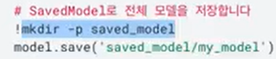
- 전체 모델 저장

# Save Model

savefile = 'saved_digits.h5'

model.save(savefile)

** ‘h5’ 확장자는 이 모델이 HDF5로 저장되었다는 것을 나타냅니다.

** 전체 모델 저장하기

: model.save 메소드를 호출하여 모델의 구조, 가중치, 훈련 설정을 하나의 파일/폴더에 저장합니다. 모델을 저장하기 때문에 원본 파이썬 코드가 없어도 사용할 수 있습니다. 옵티마이저 상태가 복원되므로 정확히 중지한 시점에서 다시 훈련을 시작할 수 있습니다.

두 개의 포맷(SavedModel과 HDF5)으로 모델을 저장할 수 있습니다. 텐서플로의 SavedModel을 로드한 다음 웹 브라우저에서 모델을 훈련하고 실행할 수 있습니다. 또는 모바일 장치에 맞도록 변환한 다음 TensorFlow Lite를 사용하여 실행할 수 있습니다.

- 모델 구조 확인

model.summary()

- 저장된 내용 확인(리눅스 명령어)

!ls -al

- 모델 불러오기

# Load Model

load_model = tf.keras.models.load_model(savefile)

** 저장된 모델로부터 새로운 케라스 모델을 로드합니다.

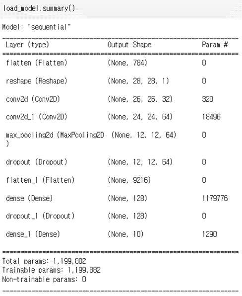
- 불러온 모델 구조 확인

load_model.summary()

- 모델 정확도 평가

# Evaluate the model using test dataset.

test_loss, test_acc = model.evaluate(test_images, test_labels)

print('Test Accuracy: ', test_acc)

- 저장했던 모델로 정확도 평가

# Evaluate the load model using test dataset.

test_loss, test_acc = load_model.evaluate(test_images, test_labels)

print('Test Accuracy: ', test_acc)

기재: 본 포스팅은 패스트캠퍼스 환급 챌린지 참여를 위해 작성되었습니다.

https://bit.ly/37BpXiC

6 ~ 7강

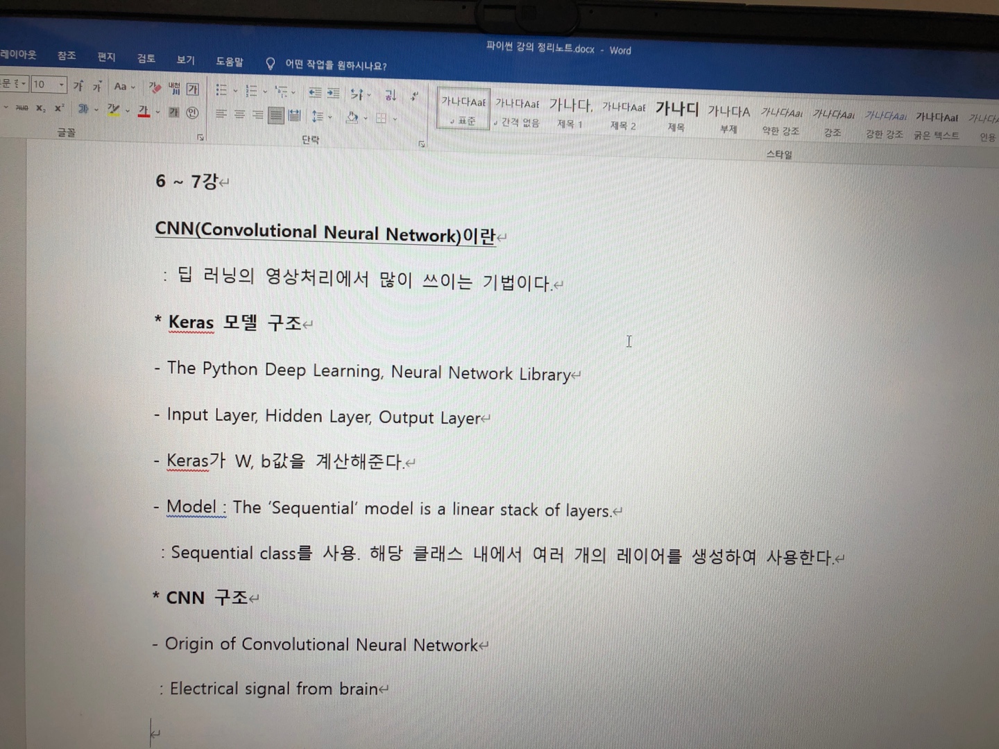
CNN(Convolutional Neural Network)이란

 : 딥 러닝의 영상처리에서 많이 쓰이는 기법이다.

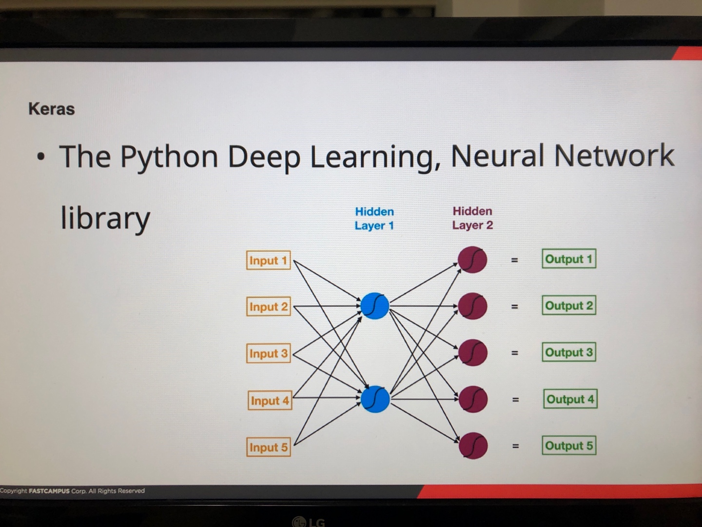
* Keras 모델 구조

- The Python Deep Learning, Neural Network Library

- Input Layer, Hidden Layer, Output Layer

- Keras가 W, b값을 계산해준다.

- Model : The ‘Sequential’ model is a linear stack of layers.

 : Sequential class를 사용. 해당 클래스 내에서 여러 개의 레이어를 생성하여 사용한다.

* CNN 구조

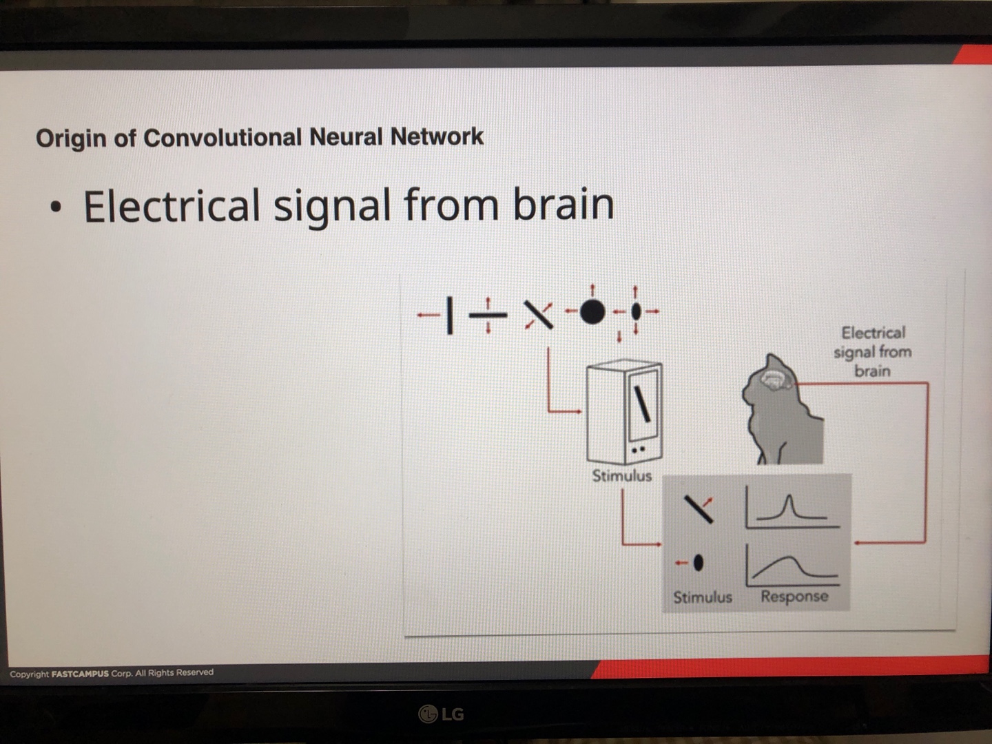
- Origin of Convolutional Neural Network

 : Electrical signal from brain

- MNIST Convolutional Neural Network

 : A class of deep neural networks, most commonly applied to analysing visual imagery.

 : 영상 분석에서 사용한다.

 : 영상 분석 중에 필요 없는 부분을 제거하고, 단순화하고, 분할하여 보면서 특성을 찾아내는 방식이다.

- Mobility Convolutional Neural Network

 : A class of deep neural networks, most commonly applied to analyzing visual imagery.

 : YOLO -> 차와 사람을 구분, 번호판 인식 등

** 영상의 노이즈를 줄이는 첫 단계는 흑백처리를 하는 것이다. 흑백처리를 통해 윤곽 같은 특성만 남겨서 단순화 하는 것이다.

* 주요 Layers

[참고] 머신러닝 용어집

https://developers.google.com/machine-learning/glossary

- 컨볼루션(Convolution)

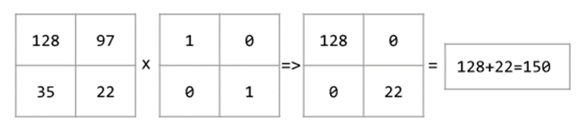
수학적으로 간단히 말하면 두 가지 함수가 섞인 것입니다. 머신러닝에서 컨볼루션은 가중치를 학습시키기 위해 컨볼루셔널 필터와 입력 행렬을 혼합합니다.

머신러닝에서 ‘컨볼루션’이라는 용어는 종종 컨볼루셔널 연산 또는 컨볼루셔널 레이어를 짧게 지칭할 때 사용됩니다.

컨볼루션이 없으면 머신러닝 알고리즘이 큰 텐서의 모들 셀에 있어서 별도의 가중치를 학습해야 합니다. 예를 들어 2,000x2,000크기의 이미지를 학습하는 머신러닝 알고리즘은 4백만 개의 가중치를 찾아야 됩니다. 컨볼루션이 있기 때문에 머신러닝 알고리즘은 컨볼루셔널 필터에 있는 모든 셀의 가중치만 찾아도 되고, 이로 인해 모델 학습에 필요한 메모리가 크게 줄어듭니다. 컨볼루셔널 필터가 적용되는 경우 모든 셀에 같은 필터가 적용되며, 각 셀에 필터가 곱해집니다.

→ 단순화 하여, 메모리 용량을 줄인다.

- 컨볼루셔널 필터(Convolutional Filter)

컨볼루셔널 연산에서 사용되는 두 가지 중 하나입니다. 다른 하나는 입력 행렬의 슬라이스 입니다. 컨볼루셔널 필터는 입력 행력과 순위(차원 수)는 동일하지만 모양은 더 작은 행렬입니다. 예를 들어 입력 행렬이 28x28인 경우 컨볼루셔널 필터는 이보다 작은 2차원 행렬이 됩니다.

사진 조작에서 사용되는 컨볼루셔널 필터는 일반적으로 1과 0으로 구성된 일정한 패턴으로 설정됩니다. 머신러닝에서 컨볼루셔널 필터는 일반적으로 난수로 채워지며 네트워크가 이상적인 값을 학습시킵니다.

→ 필터를 통해 대표 값을 찾아내고 행렬의 크기를 줄인다.

- 컨볼루셔널 신경망(Convolutional Neural Network)

 Convolutional Layer, Pooling Layer, Dense Layer

- 풀링(Pooling)

이전의 컨볼루셔널 레이어에 생성된 행렬을 작은 행렬로 줄이는 과정입니다. 풀링을 하면 보통 풀링된 영역에서 최대값 또는 평균값을 취하게 됩니다.

: Maxpooling → 대표 값을 찾는 것

→ 너무 줄어들면 Vanishing Gradient 현상이 나타날 수 있음.

→ 단순화하고 특성 값을 찾아내는 일련의 행위이다.

CNN(Convolutional Neural Network)으로 모델 강화하기

- 필요한 라이브러리 인포트

# TensorFlow and tf.keras

import tensorflow as tf

from tensorflow import keras

# Helper libraries

import numpy as np

import matplotlib.pyplot as plt

import math

- 상수 선언

# Define Constants

batch_size = 128

# 학습 횟수

epochs = 100

# 데이터를 가져오는 횟수

num_classes = 10

- MNIST에서 학습용(6만개), 테스트용(1만개) 이미지 셋(이미지, 결과 값 페어) 다운로드

: train_images는 가로 28 세로 28(28x28)의 리스트 6만개

# Download MNIST dataset.

mnist = keras.datasets.mnist

(train_images, train_labels), (test_images, test_labels) = mnist.load_data()

- Tensorflow에서 계산하기 쉽도록 값을 0에서 1사이의 값으로 변환 계산한다.

 : 실수로 계산하는 것이 더 좋다.

** 각 이미지에는 0~ 25까지의 채도 값이 들어있다.

# Normalize the input image so that each pixel value is between 0 to 1.

train_images = train_images / 255.0

test_images = test_images / 255.0

- 모델 생성

** 모델을 견고하게 변경, 은닉층을 보강, Convolutional Neural Network를 이용해서 강화

# Define the model architecture with CNN

model = keras.Sequential([

                         # Input Layer

# Flatten : 2차원배열을 1차원으로 변환해준다.

                         keras.layers.Flatten(input_shape=(28,28)),

# Hidden Layers

# Reshape : Convolutional Layer와 Pooling Layer에서 사용하기 위해 다시 2차원으로 변형한다.

                         keras.layers.Reshape(target_shape=(28, 28, 1)),

                         # Conv2D : Convolutional Layer

                         keras.layers.Conv2D(filters=32, kernel_size=(3, 3), activation=tf.nn.relu),

                         keras.layers.Conv2D(filters=64, kernel_size=(3, 3), activation=tf.nn.relu),

                         # pool_size=(2, 2) : 4(2x2)개 중에서 가장 큰 값을 뽑는다.

                         keras.layers.MaxPooling2D(pool_size=(2, 2)),

                         # Dropout(0.25) : 무작위로 25%만큼 버린다.

                         keras.layers.Dropout(0.25),

                         # 위에서 2차원으로 변형했던 것을 다시 1차원으로 변형한다.

                         keras.layers.Flatten(input_shape=(28, 28)),

                         keras.layers.Dense(128, activation=tf.nn.relu),

                         keras.layers.Dropout(0.5),

                         # Output Layer

                         keras.layers.Dense(num_classes, activation='softmax')

])

model.compile(optimizer='adam',

              loss=tf.keras.losses.SparseCategoricalCrossentropy(from_logits=True),

              metrics=['accuracy'])

** 드롭아웃 정규화(Dropout regularization)

신경망을 학습시키는 데 유용한 정규화 형태입니다. 드롭아웃 정규화를 사용하면 단일 경사 스텝이 일어날 때마다 특정 네트워크 레이어의 유닛을 고정된 개수만큼 무작위로 선택하여 삭제합니다. 드롭아웃하는 유닛이 많을수록 정규화가 강력 해집니다. 이 방식은 네트워크를 학습시켜 더 작은 네트워크로 이루어진 대규모 앙상블을 모방하도록 하는 방식과 비슷합니다.

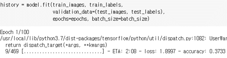
- 학습 : Validation dataset도 이용하여 결과 값의 정확도를 높인다.

history = model.fit(train_images, train_labels,

                    validation_data=(test_images, test_labels),

                    epochs=epochs, batch_size=batch_size)

- 모델 정확도 평가

# Evaluate the model using test dataset.

test_loss, test_acc = model.evaluate(test_images, test_labels)

print('Test Accuracy: ', test_acc)

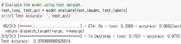
** Convolutional Layer사용 전 정확도가 97%였음.

- 그림 표시용 함수 선언

# Helper function to display digit images

# 샘플을 보여주는 함수

def show_sample(images, labels, sample_count=25):

  # Create a square with can fit {sample_count} images

  grid_count = math.ceil(math.ceil(math.sqrt(sample_count)))

  grid_count = min(grid_count, len(images), len(labels))

  plt.figure(figsize=(2*grid_count, 2*grid_count))

  for i in range(sample_count):

    plt.subplot(grid_count, grid_count, i+1)

    plt.xticks([])

    plt.yticks([])

    plt.grid(False)

    plt.imshow(images[i], cmap=plt.cm.gray)

    plt.xlabel(labels[i])

  plt.show()

# Helper function to display specific digit images

# 샘플의 특정 숫자를 보여주는 함수

def show_sample_digit(images, labels, digit, sample_count=25):

  # Create a square with can fit {sample_count} images

  grid_count = math.ceil(math.ceil(math.sqrt(sample_count)))

  grid_count = min(grid_count, len(images), len(labels))

  plt.figure(figsize=(2*grid_count, 2*grid_count))

  i = 0

  digit_count = 0

  while digit_count < sample_count:

    i += 1

    if (digit == labels[i]):

      plt.subplot(grid_count, grid_count, digit_count+1)

      plt.xticks([])

      plt.yticks([])

      plt.grid(False)

      plt.imshow(images[i], cmap=plt.cm.gray)

      plt.xlabel(labels[i])

      digit_count += 1

  plt.show()

# Helper function to display specific digit images

# 특정 숫자를 좀 더 크게 보여주는 함수

def show_digit_image(image):

  # Draw digit image

  fig = plt.figure()

  ax = fig.add_subplot(1, 1, 1)

  # Major ticks every 20, minor ticks every 5

  major_ticks = np.arange(0, 29, 5)

  minor_ticks = np.arange(0, 29, 1)

  ax.set_xticks(major_ticks)

  ax.set_xticks(minor_ticks, minor=True)

  ax.set_yticks(major_ticks)

  ax.set_yticks(minor_ticks, minor=True)

  # And a corresponding grid

  ax.grid(which='both')

  # Or if you want different settings for the grids:

  ax.grid(which='minor', alpha=0.2)

  ax.grid(which='major', alpha=0.5)

  ax.imshow(image, cmap=plt.cm.binary)

  plt.show()

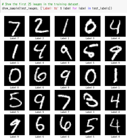
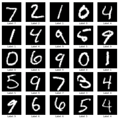
- 앞 25개의 이미지를 보여준다.

# Show the first 25 images in the training dataset.

show_sample(test_images, ['Label: %s' % label for label in test_labels])

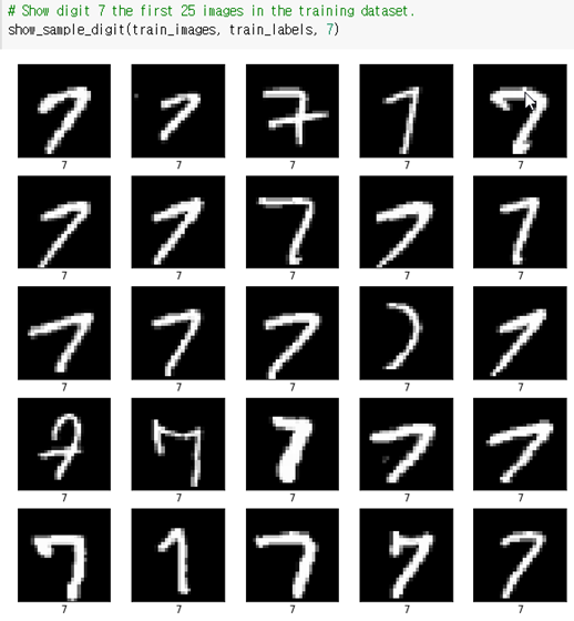
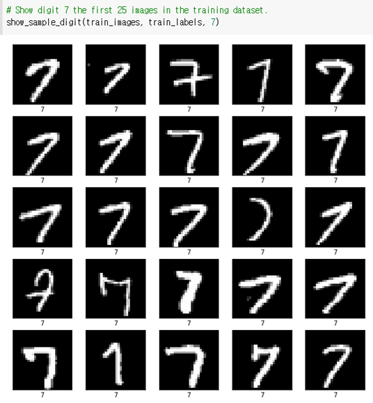
- 숫자 7의 이미지만 모아서 25개 보여준다.

# Show digit 7 the first 25 images in the training dataset.

show_sample_digit(train_images, train_labels, 7)

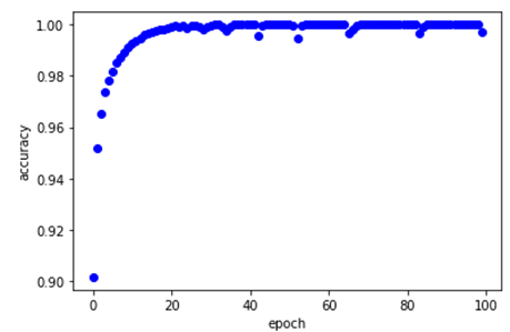
- 정확도 , Loss 값의 그래프 작성

# Evaluate the model using test dataset. - Show performance

fig, loss_ax = plt.subplots()

fig, acc_ax = plt.subplots()

loss_ax.plot(history.history['loss'], 'ro', label='train_loss')

loss_ax.plot(history.history['val_loss'], 'r:', label='validation_loss')

loss_ax.set_xlabel('epoch')

loss_ax.set_ylabel('loss')

loss_ax.legend(loc='upper left')

acc_ax.plot(history.history['accuracy'], 'bo', label='train_accuracy')

acc_ax.plot(history.history['val_accuracy'], 'b:', label='validation_accuracy')

acc_ax.set_xlabel('epoch')

acc_ax.set_ylabel('accuracy')

# location 지정

acc_ax.legend(loc='upper left')

plt.show()

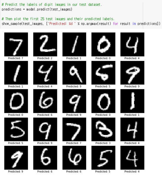
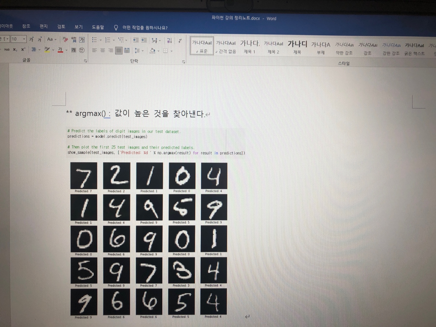
- 테스트 이미지 수만큼 결과치 예상, 예상치 정확도 상위 25개 출력

# Predict the labels of digit images in our test dataset.

predictions = model.predict(test_images)

# Then plot the first 25 test images and their predicted labels.

show_sample(test_images, ['Predicted: %d ' % np.argmax(result) for result in predictions])

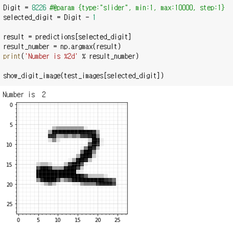
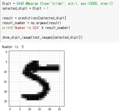
- 1만개 중 선택한 값을 보여준다.

Digit = 8226 #@param {type:"slider", min:1, max:10000, step:1}

selected_digit = Digit - 1

result = predictions[selected_digit]

result_number = np.argmax(result)

print('Number is %2d' % result_number)

show_digit_image(test_images[selected_digit])

기재: 본 포스팅은 패스트캠퍼스 환급 챌린지 참여를 위해 작성되었습니다.

https://bit.ly/37BpXiC

5강

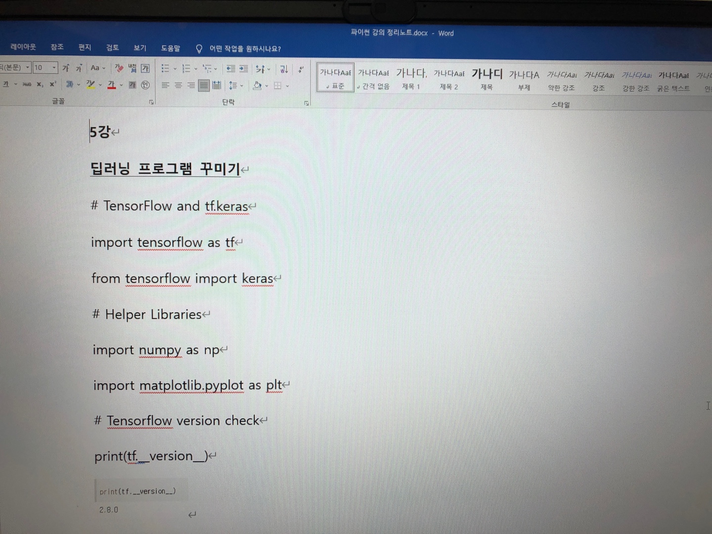
딥러닝 프로그램 꾸미기

# TensorFlow and tf.keras

import tensorflow as tf

from tensorflow import keras

# Helper Libraries

import numpy as np

import matplotlib.pyplot as plt

# Tensorflow version check

print(tf.__version__)

- 상수 설정

#Define Constants

batch_size = 128

epochs = 100

num_classes = 10

# Download MNIST dataset.

mnist = keras.datasets.mnist

(train_images, train_labels), (test_images, test_labels) = mnist.load_data()

** 이미지와 해당 이미지 값을 가져온다.

** train 이미지가 6만개, test 이미지가 1만개이다.

- Tensorflow가 계산하기 쉽게 255.0으로 나눠준다.

# Normalize the input image so that each pixel value is between 0 to 1.

train_images = train_images / 255.0

test_images = test_images / 255.0

- 모델 생성

# Define the model architecture

# Create Stack

model = keras.Sequential([

                         keras.layers.Flatten(input_shape=(28,28)),

                         keras.layers.Dense(128, activation=tf.nn.relu),

                         keras.layers.Dense(num_classes, activation='softmax')

])

# Compile

model.compile(optimizer='adam',

              loss=tf.keras.losses.SparseCategoricalCrossentropy(from_logits=True),

              metrics=['accuracy'])

** Sequential을 list형식으로 만들 수 있다.

** Flatten() : 28x28의 2차원 배열을 1차원으로 변환

** 128개의 은닉층

** activation='softmax' = activation=tf.nn.softmax 는 같은 것이다.

** SparseCategoricalCrossentropy : Multinomial Classification이기 때문

- 학습

history = model.fit(train_images, train_labels, epochs=epochs, batch_size=batch_size)

** input : train_images

** result : train_labels

** batch_size=batch_size : 몇 번 단위로 데이터를 확인할 것인지를 설정하는 것

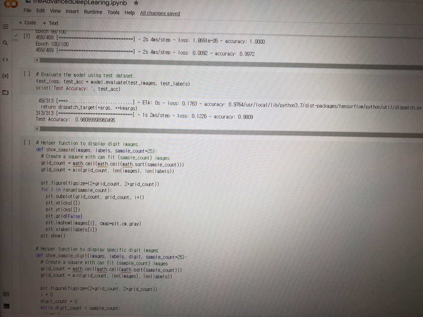
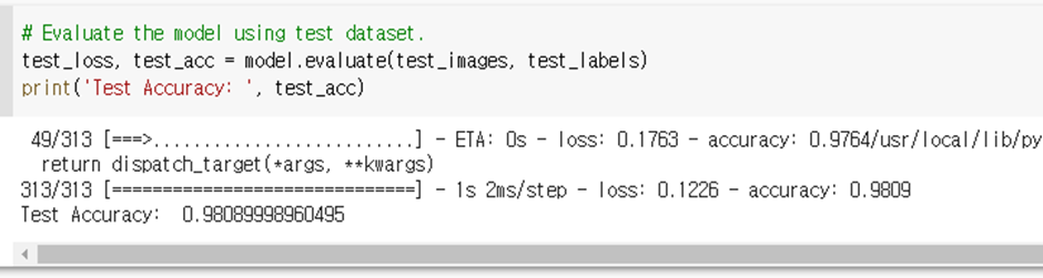
# Evaluate the model using test dataset.

test_loss, test_acc = model.evaluate(test_images, test_labels)

print('Test Accuracy: ', test_acc)

- 숫자를 보여주는 함수

import math

[참조]

https://colab.research.google.com/github/tensorflow/examples/blob/master/lite/examples/digit_classifier/ml/mnist_tflite.ipynb

- 그래프를 그리는 함수

# Helper function to display digit images

def show_sample(images, labels, sample_count=25):

  # Create a square with can fit {sample_count} images

  grid_count = math.ceil(math.ceil(math.sqrt(sample_count)))

grid_count = min(grid_count, len(images), len(labels))

** math.sqrt(숫자) : 숫자에 루트를 씌운 개수만큼 격자형태를 만든다.

ex) math.sqrt(25) : 5 x 5 의 격자형태

plt.figure(figsize=(2*grid_count, 2*grid_count))

  for i in range(sample_count):

    plt.subplot(grid_count, grid_count, i+1)

    plt.xticks([])

    plt.yticks([])

    plt.grid(False)

    plt.imshow(images[i], cmap=plt.cm.gray)

    plt.xlabel(labels[i])

plt.show()

** plt.grid(False) : 그리드가 보이지 않게 표시

** cmap=plt.cm.gray : 하얀 바탕으로 표시, default는 보라색 바탕

# Helper function to display specific digit images

def show_sample_digit(images, labels, digit, sample_count=25):

- 숫자가 7인 경우의 처리

  # Create a square with can fit {sample_count} images

  grid_count = math.ceil(math.ceil(math.sqrt(sample_count)))

  grid_count = min(grid_count, len(images), len(labels))

plt.figure(figsize=(2*grid_count, 2*grid_count))

  i = 0

  digit_count = 0

  while digit_count < sample_count:

    i += 1

    if (digit == labels[i]):

      plt.subplot(grid_count, grid_count, digit_count+1)

      plt.xticks([])

      plt.yticks([])

      plt.grid(False)

      plt.imshow(images[i], cmap=plt.cm.gray)

      plt.xlabel(labels[i])

      digit_count += 1

plt.show()

- 특정한 하나의 이미지를 보여주는 함수

# Helper function to display specific digit images

def show_digit_image(image):

  # Draw digit image

  fig = plt.figure()

  ax = fig.add_subplot(1, 1, 1)

  # Major ticks every 20, minor ticks every 5

  major_ticks = np.arange(0, 29, 5)

  minor_ticks = np.arange(0, 29, 1)

  ax.set_xticks(major_ticks)

  ax.set_xticks(minor_ticks, minor=True)

  ax.set_yticks(major_ticks)

  ax.set_yticks(minor_ticks, minor=True)

  # And a corresponding grid

  ax.grid(which='both')

  # Or if you want different settings for the grids:

  ax.grid(which='minor', alpha=0.2)

  ax.grid(which='major', alpha=0.5)

  ax.imshow(image, cmap=plt.cm.binary)

plt.show()

- 테스트용 이미지를 가져옴

# Show the first 25 images in the training dataset.

show_sample(test_images, ['Label: %s' % label for label in test_labels])

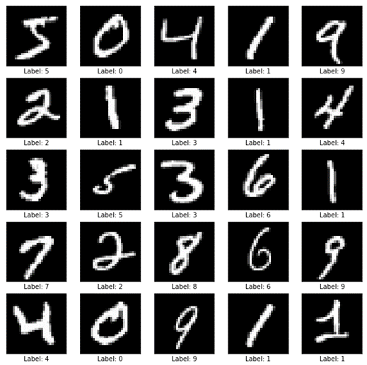
- 학습용 이미지 확인

# Show the first 25 images in the training dataset.

show_sample(train_images, ['Label: %s' % label for label in train_labels])

- 숫자 7의 외국 표기법이 다름. 숫자 7의 이미지를 가져오게 함.

# Show digit 7 the first 25 images in the training dataset.

show_sample_digit(train_images, train_labels, 7)

- 모델 평가

# Evaluate the model using test dataset. - Show performance

fig, loss_ax = plt.subplots()

fig, acc_ax = plt.subplots()

# Loss용 그래프

loss_ax.plot(history.history['loss'], 'ro')

loss_ax.set_xlabel('epoch')

loss_ax.set_ylabel('loss')

# Accuracy용그래프

acc_ax.plot(history.history['accuracy'], 'bo')

acc_ax.set_xlabel('epoch')

acc_ax.set_ylabel('accuracy')

** ro : red의 o모양

** bo : blue의 o모양

** Loss는 점점 줄어들고 Accuracy는 점점 증가한다.

- 전체 테스트 데이터를 가지고 예측

# Predict the labels of digit images in our test dataset.

predictions = model.predict(test_images)

# Then plot the first 25 test images and their predicted labels.

show_sample(test_images, ['Predicted: %d ' % np.argmax(result) for result in predictions])

** 테스트 이미지 1만개를 전부 예측하고, 그 중 제일 정확도가 높은 상위 25개만 표시한다.

** argmax() : 값이 높은 것을 찾아낸다.

Digit = 8448 #@param {type:"slider", min:1, max:10000, step:1}

selected_digit = Digit – 1

# 실제 리스트 상에서는 0번째이므로 -1로 계산해준다.

result = predictions[selected_digit]

result_number = np.argmax(result)

print('Number is %2d' % result_number)

show_digit_image(test_images[selected_digit])

기재: 본 포스팅은 패스트캠퍼스 환급 챌린지 참여를 위해 작성되었습니다.

https://bit.ly/37BpXiC

4강

첫 딥러닝 프로그램

* 딥러닝의 이해

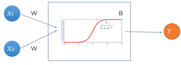
- 퍼셉트론(Perceptron) : 입력, 함수, 출력이 있는 구조

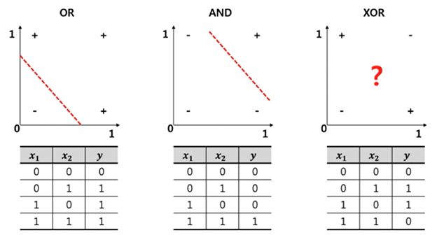
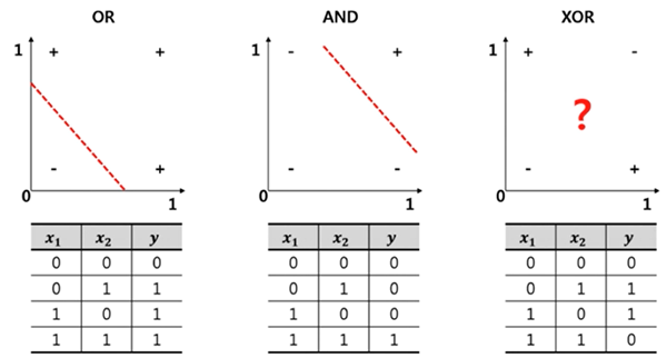
- 단수 퍼셉트론으로는 XOR문제를 해결하지 못한다.

→ 다층 퍼셉트론으로 XOR문제를 해결한다.

- Back propagation : 가중치 조절 방법

- Vanishing Gradient : 레이어 수가 너무 많으면 가중치가 사라지기도 한다.

- Keras : The Python Deep Learning, Neural Network Library

* Keras 모델 구조

- Model : The ‘Sequential’ model is a linear stack of layers.

- Model Summary, prints a summary representation of your model

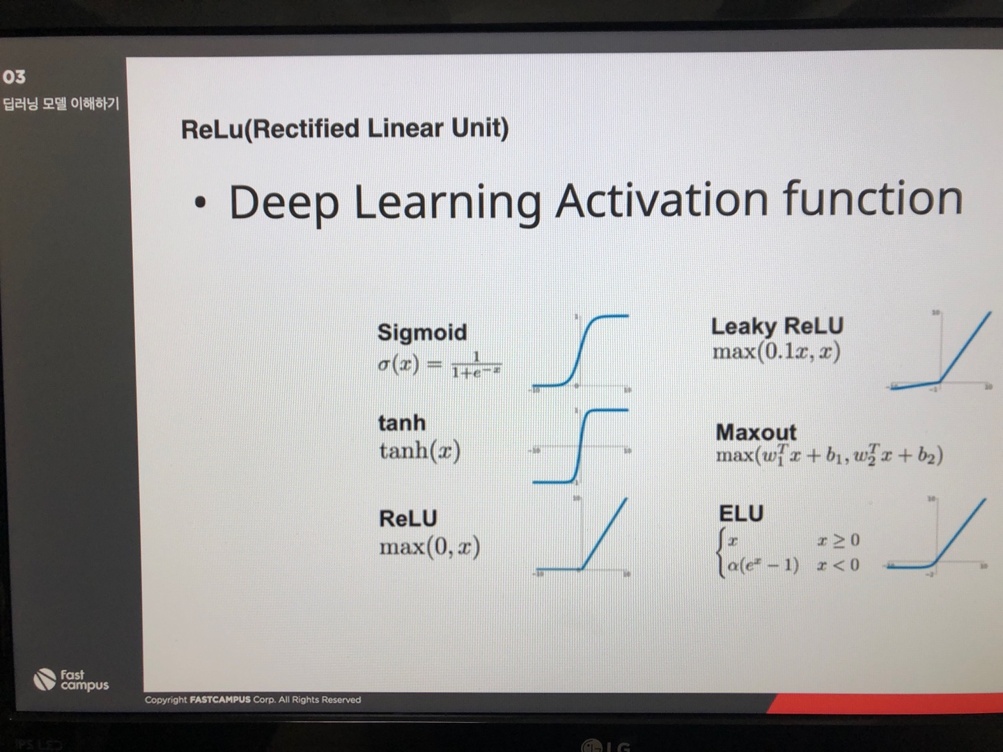
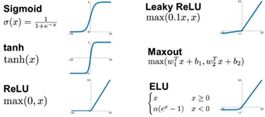
* ReLu(Rectified Linear Unit)

- Sigmoid는 0부터 1사이의 값을 다루는데, 이 경우 0에 가까운 값이 사라지는 현상이 발생하므로 Sigmoid가 아니라 ReLu 함수를 사용한다.

- Deep Learning Activation Function

* 코딩

# TensorFlow and tf.keras

import tensorflow as tf

from tensorflow import keras

# Helper Libraries

import numpy as np

import matplotlib.pyplot as plt

# Tensorflow version check

print(tf.__version__)

- 상수 설정

#Define Constants

batch_size = 128

epochs = 100

num_classes = 10

- MINIST

MNIST 데이터베이스 (Modified National Institute of Standards and Technology database)는 손으로 쓴 숫자들로 이루어진 대형 데이터베이스

# Download MNIST dataset.

mnist = keras.datasets.mnist

(train_images, train_labels), (test_images, test_labels) = mnist.load_data()

** 이미지와 해당 이미지 값을 가져온다.

# Normalize the input image so that each pixel value is between 0 to 1.

train_images = train_images / 255.0

test_images = test_images / 255.0

- 모델 생성

# Define the model architecture

# Create Stack

model = keras.Sequential([

                         keras.layers.Flatten(input_shape=(28,28)),

                         keras.layers.Dense(128, activation=tf.nn.relu),

                         keras.layers.Dense(num_classes, activation='softmax')

])

# Compile

model.compile(optimizer='adam',

              loss=tf.keras.losses.SparseCategoricalCrossentropy(from_logits=True),

              metrics=['accuracy'])

** Sequential을 list형식으로 만들 수 있다.

** Flatten() : 28x28의 2차원 배열을 1차원으로 변환

** activation='softmax' = activation=tf.nn.softmax 는 같은 것이다.

** SparseCategoricalCrossentropy : Multinomial Classification이기 때문

- 학습

history = model.fit(train_images, train_labels, epochs=epochs, batch_size=batch_size)

** input : train_images

** result : train_labels

** batch_size=batch_size : 몇 번 단위로 데이터를 확인할 것인지를 설정하는 것

batch_size가 많으면 그만큼 로드 시간이 오래 걸린다. 메모리 사용과 관련이 있음.

일종의 되새김 효과라고 할 수 있다.

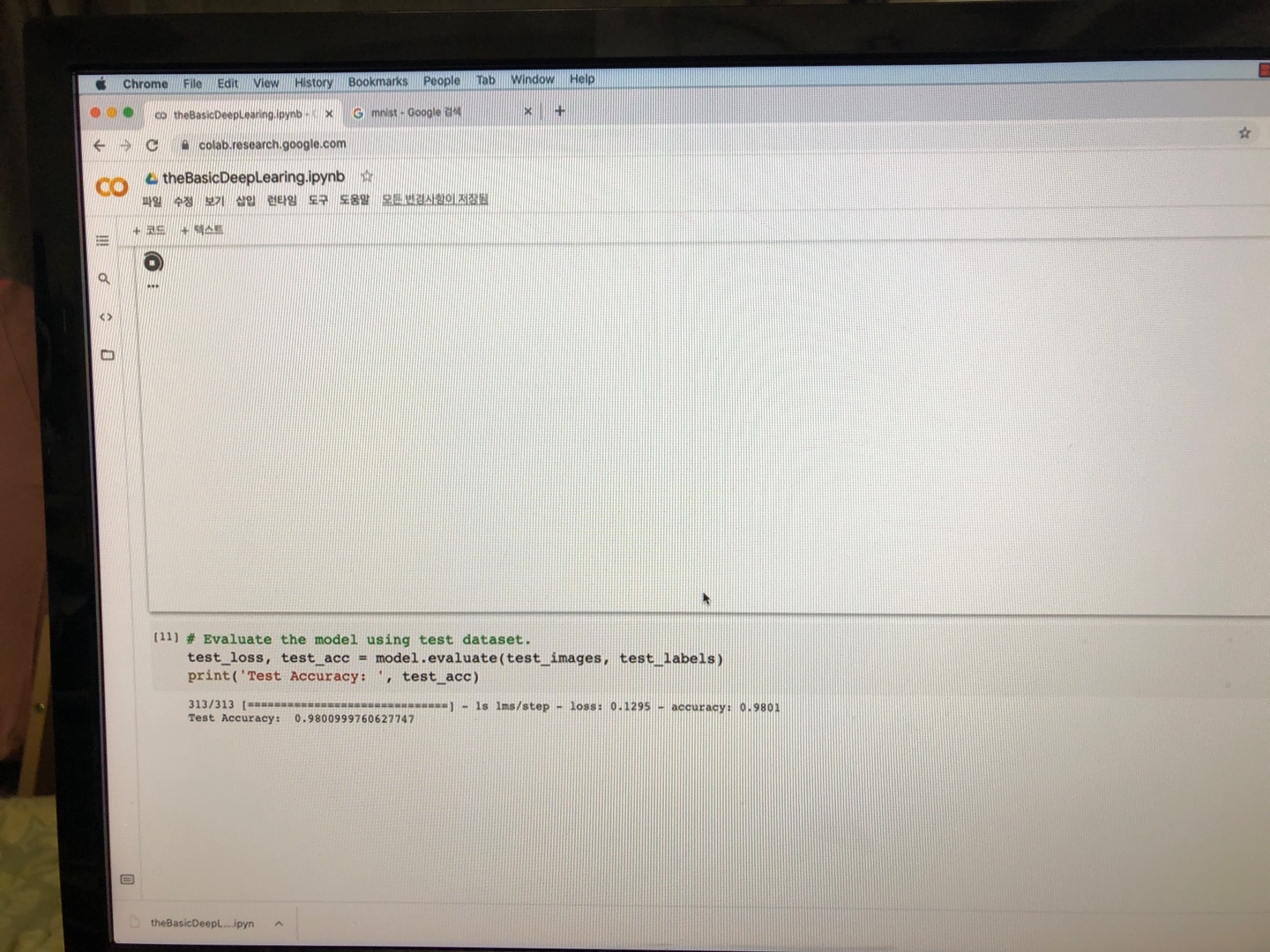
# Evaluate the model using test dataset.

test_loss, test_acc = model.evaluate(test_images, test_labels)

print('Test Accuracy: ', test_acc)

학습결과 정확도가 98%이다.

기재: 본 포스팅은 패스트캠퍼스 환급 챌린지 참여를 위해 작성되었습니다.

https://bit.ly/37BpXiC

3강

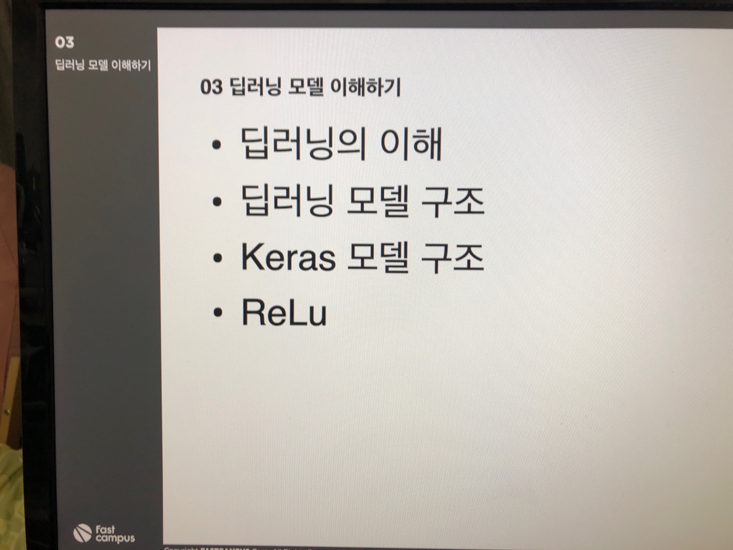
딥러닝 모델 이해하기

* 딥러닝의 의해

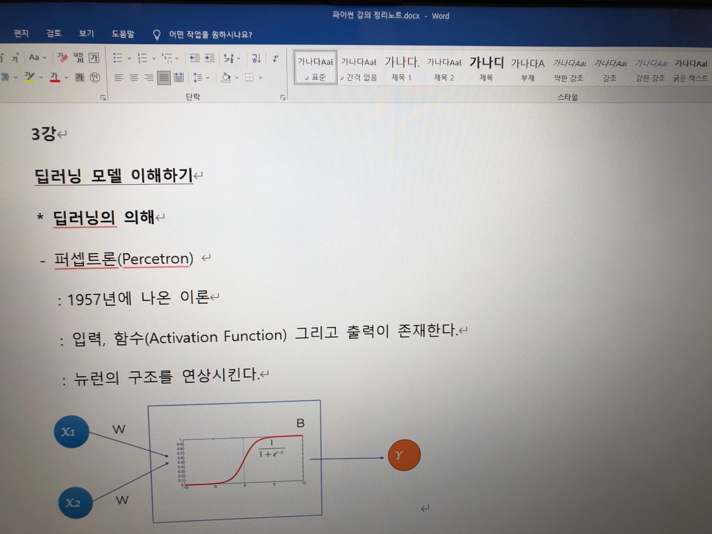
- 퍼셉트론(Percetron)

: 1957년에 나온 이론

: 입력, 함수(Activation Function) 그리고 출력이 존재한다.

: 뉴런의 구조를 연상시킨다.

- XOR(Exclusive OR) Problem

 : (한 개의)퍼셉트론으로는 XOR문제를 해결하지 못한다.

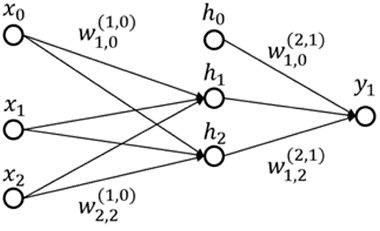
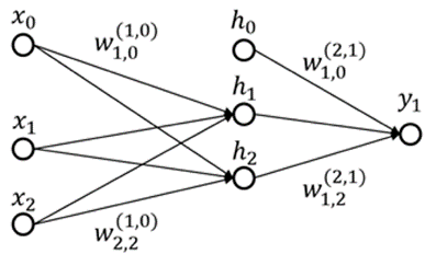
- Multi Layer Perceptron

 : 다층 퍼셉트론으로 XOR문제를 해결한다.

 : (MIT Marvin Minsky) W, b값이 각각 존재하고, 그 사이의 상관관계가 완벽하게 맞아떨어지게 하는 것은 어렵지 않나?

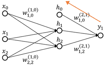
- Back propagation

 : Back propagation으로 가중치를 조정한다.

 : 계산하면서 뒤에서 결과 값에 따라 가중치를 조정하면 되지 않은가.

- Vanishing Gradient

 : Layer가 많아지면 가중치가 사라지기도 한다.

 : Layer가 많다고 좋은 것은 아니다.

* 딥러닝의 모델 구조

- Keras

 The Python Deep Learning, Neural Network library

Tensorflow2의 중요 구성 요소

Multi-Layer 구현에 좋다.

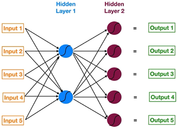
 Multi Input Layer, Hidden Layer, Multi Output Layer

* Keras 모델 구조

- Model(Keras의 Class) – The ‘Sequential’ model is a linear stack of layers.

: Sequential model : 선형으로 Layer가 하나씩 쌓아 나가는 구조

- Input Layer(Single/Multi), Hidden Layer(None/Single/Multi), Output Layer(Single/Multi)가 존재한다.

 언급된 3개의 Layer를 적층 하는 방식.

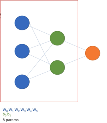
- Model Summary, prints a summary representation of your model.

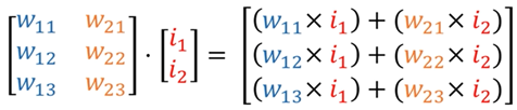
 8 params : W와 b에서 나온 선의 개수의 합

* ReLu 레루 Activation Function(함수)

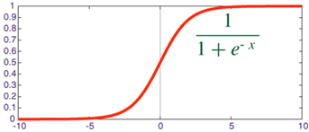
- Sigmoid(Binary Classification)

 극단치(예외적으로 발생하는 값)가 존재하는 경우, 극단치를 없애서 평균값에 영향을 미치지 않도록 하기 위함.

 0부터 1까지의 값이 존재함.

Sigmoid의 경우 Vanishing Gradient현상이 생기기 쉬움

 0과 1사이의 값만 존재하므로 확률적으로 0에 가까운 값이 더 많음. 그리고 0에 가까운 값은 사라지기가 쉬움.

- ReLu(Rectified Linear Unit) : Deep Learning에서 Sigmoid함수보다 잘 사용되는 함수

 Deep Learning Activation function

 0보다 큰 값은 그대로 존재, 0인 값의 경우 없애서 Vanishing Gradient 현상을 상쇄한다.

기재: 본 포스팅은 패스트캠퍼스 환급 챌린지 참여를 위해 작성되었습니다.

https://bit.ly/37BpXiC

Part4. 딥러닝 영상처리 Basic to Project

Ch 01. 딥러닝 기본 익히기

1강

딥러닝 강의소개

* 첫 딥러닝 프로그램

* CNN(Convolutional Neural Network)이란?

* Keras Tuner 사용하기

* Colab에서 OpenCV사용하기

* Haar-cascade Detection이란?

* YOLO(You Only Look Once) 사물 식별(Object Detection) 프로그램

* 차와 차량 번호판 식별

* 동영상에서 차선을 인식하기

2강

딥러닝의 등장

* 인공지능, 머신러닝, 딥러닝

- 인공지능 Artificial Intelligence

A technique which enables machines to mimic human behavior.

- 머신러닝 Machine Learning

  Subset of AI technique which use statistical methods to enable machines to improve with experience.

통계치/경험을 이용한 방법

- 딥러닝 Deep Learning

Subset of ML(Machine Learning) which make the computation of multi-layer neural network feasible.

- 인공지능 역사

* 머신러닝 요약

- 선형회귀 Linear Regression 문제해결 방법 (Problem Solving Procedure)

1) Hypothesis of Linear Regression 가설 설정

 Linear regression is a linear approach to modeling the relationship between a scalar response.

 Y = ax + b → H(x) = Wx + b

2) Cost of Linear Regression

 Cost function means how fit the line to actual data.

 H(x) – y

3) Minimize Cost

 Find the minimal cost and get the right W(Weight) and b(bias).

 Minimize cost(W,b)

- Multi Variable Problem Solving Procedure

 : Hypothesis, Cost with n Variables Input and n Output

1) Hypothesis

H(x1, x2, x3…) = W1x1 + W2x2 + W3x3… + b

2) Cost

cost(W,b) = sum(H(x1, x2, x3…) – y)2

* 딥러닝의 이해

- 퍼셉트론(Perceptron)

 : 입력, 함수 그리고 출력이 있는 구조

- 퍼셉트론(Perceptron), 신경망(Neural Network)

 퍼셉트론의 컨셉이 뇌의 구조와 유사하다.

 뉴런은 자극을 받아서 반응한다. 뉴런의 뭉치인 시냅스가 모여서 사람이 사고하는 모양이, 여러 개의 퍼셉트론이 모여서 결과값을 출력하는 것과 유사하다.

- XOR(Exclusive OR) Problem

 퍼셉트론으로 XOR문제를 해결 못 한다.

- Multi Layer Perceptron

: 다층 퍼셉트론으로 XOR문제를 해결한다.

- Back propagation

 Back propagation으로 가중치를 조정한다.

- Vanishing Gradient

 Layer가 많아지면 가중치가 사라지기도 한다.

 그래서 정확한 값이 나오지 않는 경우도 생긴다.

 그러므로 은닉층이 많을수록 좋은 것은 아니다.

기재: 본 포스팅은 패스트캠퍼스 환급 챌린지 참여를 위해 작성되었습니다.

https://bit.ly/37BpXiC